Blog

QT GUI Widgets with Message Passing

 Just today, I issued a Pull Request for a new feature in GNU Radio. This adds a new form of what we already called the QT GUI Entry widget. That widget provides a simple QLineEdit box where we type in values, they get stored as a Python variable, and we pass these variables around like normal GRC variables. When running, updates to the entry box are propagated to anything using that variable in the flowgraph.

We're trying to move beyond this world where everything is in a Python file that's assumed to be completely local. Instead, we want to move to a world where we can use the message passing architecture to manage data and settings. So when we have a message interface to a block, we might want to post data or update a value through that message interface from a UI somehow. This leads us to the possibility that the UI is a separate window, application, or even machine from the running flowgraph. We have already made strides in this direction by adding the postMessage interface to ControlPort, which I spoke about in the last post on New Way of Using ContorlPort. However, ControlPort can take some time to set up the application, craft the UI, and make a working product. Aside from that method, we wanted to have easy ways within GRC to build applications that allow us to pass and manage messages easily. Hence the new QTGUI Message Edit Box (qtgui_edit_box_msg).


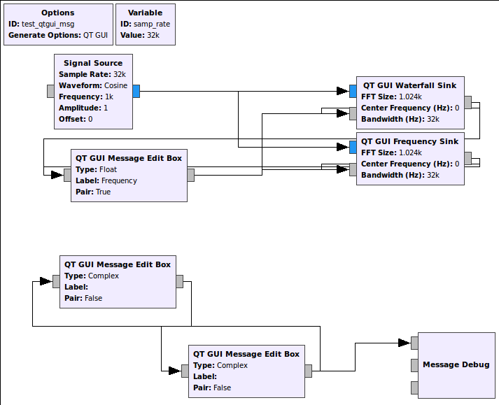
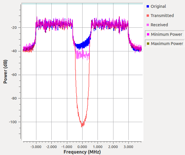
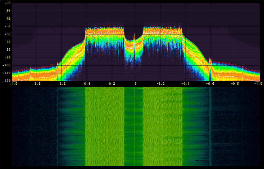
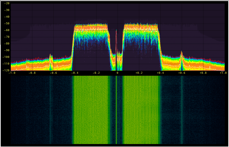
This is an flowgraph example that now comes with GNU Radio's gr-qtgui (test_qtgui_msg.grc). This shows the use of three of the new message edit boxes. In the upper part of the graph, we have the edit box controlling the center frequency of a Waterfall and Frequency Sink. These sinks can take in a message that's a PMT pair in the form ( "freq" <float frequency> ). So the edit box has a setting called Pair that sets this up to handle the PMT pair messages. It's actually the default since we'll be using the key:value pair concept a lot to manage message control interfaces. When the edit box is updated and we press enter, it publishes a message and the two GUI sinks are subscribed to them, so they get the message, parse it, and update their center frequency values accordingly.

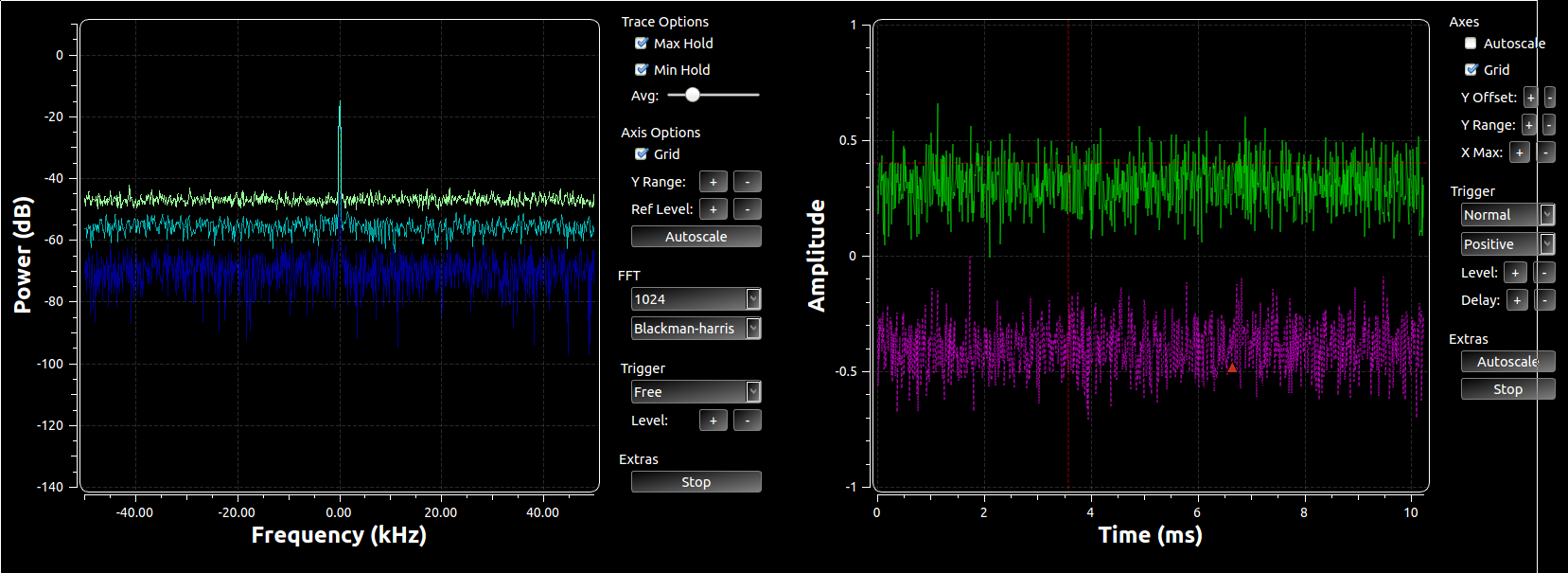
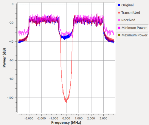
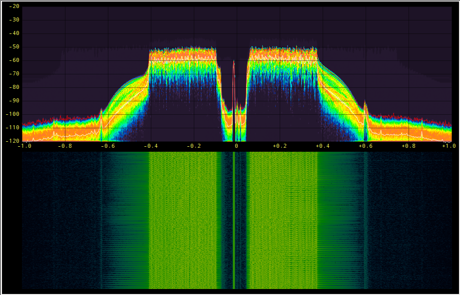
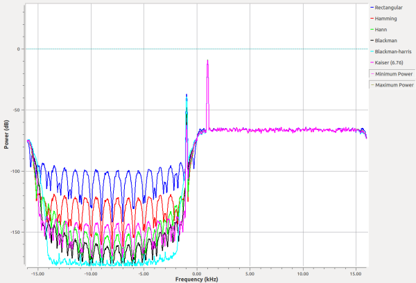
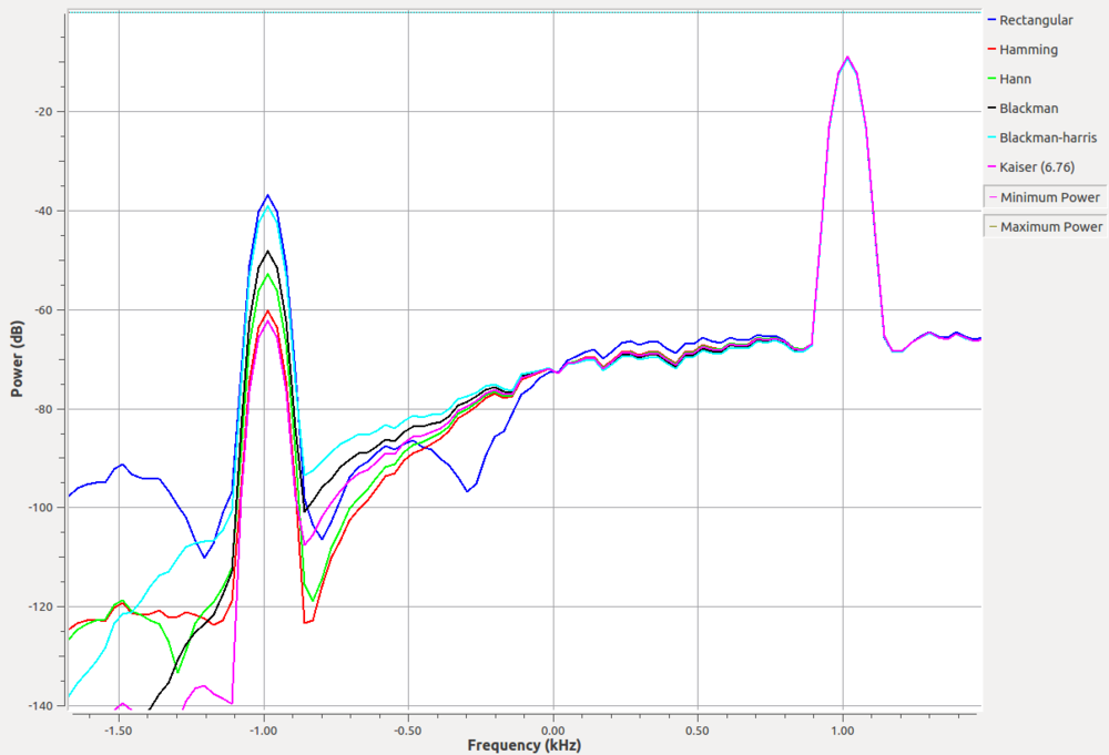
Now the flip side of this is that the edit boxes also have an input message port. This allows us to programmatically set the value inside the box. The two GUI sinks have the ability to have a user adjust their center frequency. When a user double-clicks on a frequency in the plot, the block sets that value as the center frequency and then publishes a message (in the same key:value pair where key="freq"). This means that not only is the widget we just double-clicked updated, anything listening for that message is updated. So the edit box is kept in sync with the change in the GUI. Now, when the new data received is different than what was in that edit box to begin with, the box re-emits that message. So now, say we double-clicked on the Frequency Sink near the 10 kHz frequency line. That message is propagated not only to the edit box, but the message also gets sent from that box through to the waterfall sink. Now all of the widgets are kept in sync. And because the re-posting of the message only happens when a change occurs, we prevent continuous loops. Here's the output after the double-clicking:

Both GUI display widgets have the same center frequency, and that value is also shown in the Frequency edit box above. Because it's using the pair concept, we have two boxes, the left for the key and right for the value.

This example has two other edit boxes that show up at the bottom of the GUI. This is to allow us to easily test other properties and data types. They are connected in a loop, so when one is changed, the other immediately follows. Note here that we are not using the pair concept but that the data type is complex. To make it easy on us, we use a Boost lexical_cast, which means we use the format "(a,b)" for the real and imaginary parts. All of this, by the way, is explained in the blocks'd documentation.

Now, we have the ability to pass messages over ZMQ interfaces. Which means we can create flowgraphs on one side of the ZMQ link that just handle GUI stuff. On the other side, we use ZMQ sources to pass messages around the remotely running flowgraph. Pretty cool and now very easy to do in GRC.

This is just one way of handling QT widgets as message passing blocks. Pretty easy and universal for sending messages with data we're used to. But it's just a start and a good template for other future widgets to have similar capabilities, like with range/sliders, check boxes, combo boxes, etc. All of these should be able to pretty easily use this as a template with different GUI widgets for manipulating the actual data.

New Way of Using ControlPort

We've started down the path of providing more capabilities with ControlPort. Specifically, I'd like to get us to have more blocks within the GNU Radio main source code that support configuration over ControlPort. We are going to rely heavily on ControlPort for our Android work where the Java application space will talk to and control the running GNU Radio flowgraph almost solely over ControlPort.

One of the main things missing from our ControlPort capabilities here is the ability to control the settings of a UHD device. The main reason is that the generic interface for ControlPort comes in two forms:

  • <type> getter_method(void);
  • void setter_method(<value type> <value>);

This interface does not work for the UHD interface for most of the important parameters. For example, setting the frequency of a USRP source looks like:

tune_result_t set_center_freq(double freq, size_t chan)

So it takes two arguments and returns a data structure. This kind of thing isn't easily encompassed in ControlPort's generic interfaces.

However, instead of trying to expand the interfaces for all of these types of commands, we have one more general format interface that we can use for lots of these things, the message handler, which looks like:

  • void message_handler_function_name(pmt::pmt_t message);

It just makes sense to make use of these already-available message handling functions in blocks to handle setting values over ControlPort as well. So I've recently added a new interface to our ControlPort system called "postMessage". This function takes three arguments:

  • alias: the block's alias in the system as a serialized PMT string.
  • port: the port name of the block's message handler as a serialized PMT string.
  • msg: the actual message to be passed to the message handler as a serialized PMT.

The msg PMT can be any form of a PMT that would be created especially for the type of message expected by the message handler. All of this can be easily constructed in Python or any other supported language. In fact, in Python, we use our RPCConnection abstracted interface to take these values in as a (string alias, string port, PMT message) -- internally, these are serialized and posted to ControlPort. For example, if we have a copy block that we want to enable the copy function, we would use the following postMessage to send to block named "copy0" on the enable message port "en" with a PMT True value.

radioclient.postMessage("copy0", "en", pmt.PMT_T)

Let's take a more complicated example where we are trying to change the frequency of a USRP source. First, we have to know the alias of the USRP source in the flowgraph. As an aside, I'm hoping to provide some discovery mechanisms for available handlers exported through ControlPort soon. In our case, let's assume the alias is 'usrp_source0,' and we know from the manual that it has a port named 'command' that takes a key:value pair. One command key is 'freq' to set the frequency based on a floating point value. We've already created the ControlPort radio interface, called 'radio' here, so we just need to do:

radio.postMessage('usrp_source0', 'command',
  pmt.cons(pmt.intern('freq'), pmt.from_double(101e6)))

The only tricky thing here is to know that the command takes a PMT pair of a string and the correct value. The pmt.cons constructs a pair with the 'freq' as the first part and a double PMT for 101 MHz. This would get posted to the USRP devices to change the channel over our remote ControlPort interface.

Examples

I have added a couple of simple examples to GNU Radio to exercise this new feature. First is the simple_copy.grc file that runs a graph that has a copy block. We can use the simple_copy_controller.py program to toggle the copy block's enable port either True or False to start and stop data flowing.

The second and more exciting example is the usrp_source_control.grc. This just runs a flowgraph where data is sourced from a USRP device and plotted in time and frequency. It is set up with a sample rate of 1 MHz, but no gain, frequency, or antenna are selected as shown below.

initial_grc_setup.png

We expect to see nothing since we have no tuning or gain set, and in my case, there is no antenna connected to the default RX2 port. In the running flowgraph, we've provided no application controls for this like QTGUI slider or chooser widgets.

But since we have a ControlPort endpoint available on localhost port 9090, we can control it remotely. In this case, I'm using the program on the same machine and talking over the localhost interface.

I've used the usrp_source_controller.py application to issue ControlPort commands that will post a message to set the frequency, gain, antenna port, and sample rate to the USRP device allowing me to see the signal now shown above.

This new interface should prove to be quite powerful in controlling GNU Radio flowgraphs over ControlPort. It will also force us to expand the available message handling support on many blocks that we will be wanting to manipulate over ControlPort and in Android apps. The use of the message passing infrastructure also means we have a lot more flexibility in structuring our ControlPort commands.

FOSS SDR at W@VT

Hey, that title's not annoying at all, is it? This post discusses our forum on Free and Open Source Software (FOSS) for Software Defined Radio (SDR) at the Wireless@VT (Virginia Tech) Symposium a couple of weeks ago.

We brought together five speakers from different areas to talk about how FOSS works in their world of radio and SDR. I talked about the GNU Radio project, Philip Balister spoke on OpenEmbedded and how we use it for SDR development on embedded systems, Tim O'Shea from the Hume Center of Virginia Tech talked on their use of FOSS in research in both wireless and machine learning, Rick Mellendick from Signals Defense spoke about how FOSS has enabled work in wireless security and penetration testing, and Ben Hilburn from Ettus Research was there to speak about his perspectives on FOSS from an industry point of view.

The main intent behind this tutorial was to expose the audience to a lot of projects and tools as well as ideas that the FOSS world can offer. The various perspectives on this were to showcase how wide-reaching FOSS is in technology, business, concepts, and intent. Essentially, we wanted to help add to the discussion about how the tools and technology can impact work in various fields.

There is a lot of misunderstanding about FOSS in our world. In the world generally, sure, but I am specifically talking about wireless and signal processing where we are not brought up on open source. We see the misunderstanding as well as mistrust of it from traditional engineers and engineering. It is often seen as something that's fun as a toy or hobby, but not for real work. Plus the big question of monetization. In the five talks in the panel, I think we exposed a lot of powerful FOSS technology and projects as well as explained some of the behavior and philosophy of FOSS. You can download the presentations in the list of talks below.

I also really want to apologize publicly again to Ben Hilburn for running out of time. I completely misjudged how much time we had available, but he's been gracious enough to provide his slides here.


QTGUI Tools and Tips

It's been made apparent to me that not everyone knows about all of the capabilities in the QTGUI plotting tools we have in GNU Radio. We've also recently added a number of features that I think people will find really useful and wanted to expose here. I'll focus on just the time and frequency plots, but you'll also find a constellation plot (real and imaginary), a waterfall plot, a histogram, a raster, a generic vector plot, and a number sink.

Drop-down Menus

Each QT sink has a set of control that are specific to controlling each graph, though they share many common attributes. To access the drop-down menu, use the middle mouse button, which in cases of two-button mice might be a ctrl+click or clicking both mouse buttons together. The mouse wheel often acts as the middle mouse button. There's been some call for changing this to the right mouse button, which I'm sympathetic to, but I think we'll want to review all mice interactions to see what makes sense for everything. But for now and through v3.7.7 at least, it's the middle mouse button.

This shows the menu options for the time plot (if you can read it; my resolution is pretty high on my screen). You can set the line properties such as colors, width, markers, and style. Set the number of points to plot, change to log scale for either or both axes, turn it to a stem plot, or set the trigger options.

Some of the common properties to the graphs is the ability to start and stop the plotting, autoscale the y-axis, and save the image to file. The time, frequency, and constellation plots also have the ability to trigger off of the incoming signal. You can set the trigger to free (no triggering), auto (trigger off an event but update the plot after a time anyways), or normal (only update when the trigger hits). For the constellation and time plots, there is even the option to trigger off a specific stream tag. You can then set the level of the trigger event, the channel to trigger off of, and a few other standard triggering attributes. For the time and frequency plot, we now (as of v3.7.7) display a dashed red line to show where the triggering will occur.

There are plenty of options here to look into and play around with once you know that drop-down menu exists.

QSS Files

If you've used the QT GUI plotters before, the above graph might look a bit odd to you. You're probably used to seeing it as a white background with blue and red lines drawn on it. Well, the plotters can actually have most of their attributes controlled by a QT Style Sheet (QSS file). You install them by simply editing your GNU Radio config file. Either edit or create a new $HOME/.gnuradio/config.conf file and add the following:

[QTGUI]
qss = $prefix/share/gnuradio/themes/alt.qss

Where $prefix is the installation prefix you installed GNU Radio into (often /usr or /usr/local). Below is a look at the normal, non-qss frequency plot versus the alt.qss plot that's installed with GNU Radio.

QTGUI Frequency Plot without a QSS file used.

QTGUI Frequency Plot without a QSS file used.

QTGUI Frequency plot with alt.qss file used.

QTGUI Frequency plot with alt.qss file used.


Control Panel

We just recently added control panels to the time and frequency sinks. We will be continuing to roll out this concept to the other plots as well, but these were the first two to get the attention. The control panel is a set of widgets on the right-hand side of the graph to provide very quick and easy access to manipulating the look of many of the plot properties. You can see in the image below that we can adjust things like the x and y axis limits, do an autoscale, toggle things like min/max hold or the grid, and adjust the triggers. For the time plots, the autoscal check box turns on continuous autoscaling of the plot based on the latest set of samples while the button just does a one-shot autoscale and then holds the y-axis from there.

We can also toggle this on and off. One of the reasons I did not have this in the first place was that it takes up a lot of plotting real estate on the screen. However, when manipulating the plots, it is definitely much easier to use these tools than the drop-down menu for many of the purposes -- setting the trigger is a good example. Still, we can actually enable and disable the control panels as we need them. We can do this in GRC by going into the properties box for the plotters and setting the Control Panel option in the Config tab to Yes or No. At runtime, the drop-down menu has the option of enabling or disabling the control panel as well, so you can use it and hide as you need.

Legend

Another brand new feature is the ability to turn the plotter legends off. Tim O'Shea requested this feature, and it really seemed like a good idea. The lines in a plot are labeled, and those labels show up in a legend on the right-hand side. When plotting a lot of lines together, this can be really useful to distinguish them and present the results to others. See my recent post on the new LDPC and TPC codes and the BER plot. There, we use the legend to show which line is for which FEC technique. However, often we just plot a single line, in which case the legend just takes up an unfortunate amount of space. So now, in the GRC properties box under the Config tab for each QTGUI plotter, we can toggle the legend on or off. This cannot be done at runtime, however. Below is an image of two QTGUI time plotters showing the same signals. The one on the right has the legend on and the other has it off. This shows how much less of the display is wasted by a legend that, in this instance, doesn't tell us much about what's being plotted.

The only plotter that works differently than the rest The waterfall plot just removes the intensity legend on the right-hand side. You won't be able to relate the colors to specific power levels, but often we just need to get a glimpse of the signals and have an understanding of the relative power levels, not the exact numbers.

Working with UHD static library

Introduction

We have recently been working to support building and using static libraries for all GNU Radio components, which therefore means static libraries for our different dependencies as well. Part of this is to better support Android development work in GNU Radio, but there are other use-cases where people find it useful to build static applications for easier distribution and configuration control of systems. Whatever your feelings here, we want to support the capability.

Ettus Research will soon be updating the UHD library to also support building and using static libraries, though there are a couple of caveats. First, I'll go over some of the issues with static libraries and what we've done in GNU Radio. I'll then introduce the way they have handled it in the UHD library, which leads to other issues with libraries, at least in Ubuntu due to some decisions they have made. We'll cover these issues and show how to get around them, at least for right now.

As of the writing of this post, the static library support is not part of the mainline source code for UHD, so when I say "look at the UHD manual," I mean the future manual when they merge this concept into their distribution and release it in a future version.

GNU Radio and Static Libraries

One of the biggest issue that you run into with static libraries is in dealing with global variables. When you're doing shared library linking, you don't have to think about this, and so you can easily get lazy. We generally don't have too many of these kinds of variables as they are considered bad practice, but sometimes they are exactly what's required. The problem comes when you directly reference one of these variables. In a statically-linked library, there is no guarantee that the variable will be initialized before being called. So instead, we provide access functions for these variables. Where we might have had:

static int some_variable;

We switch to:

int get_some_variable()
{
static int some_variable = init_me;
return some_variable;
}

The difference is that when you call 'get_some_variable()' the first time, it will initialize the variable for us as a static variable. All calls after that will return the same static variable we have defined here. And then we jump through some hoops to provide access to the some_variable in another way -- like with a #define that maps to the call get_some_variable().

In GNU Radio, we have been patching it to remove any direct calls to global variables using the above method. Doing so makes it possible to build and use a libgnuradio-<component>.a file to build statically-built applications. We've supported the building of static libraries in GNU Radio for a while, now, by using the -DENABLE_STATIC_LIBS=True as a CMake argument. When this flag is enabled, we build both the shared and static libraries. So, for instance, we will build a libgnuradio-runtime.so and libgnuradio-runtime.a.

However, we do not build static versions of gr-fcd or gr-uhd because of underlying problems with the hardware libraries themselves. We did not have a static library for libuhd.a that we could use in order to statically link with libgnuradio-uhd.a. So we kept those disabled during the static library build.

Static UHD Library

Working with Ettus Research, they have added their own -DENABLE_STATIC_LIBS flag when building libuhd. This is a big help to us as we can now enable static libraries for gr-uhd. However, this one comes with a bit of a caveat and the reason for this post. LibUHD still uses static globals like I discussed above. Some of these are tied pretty tightly into the code, and so the task of updating the code is a bit more difficult. At least here, though, we have another way around it, and I felt it was worth publishing the way to handle it here.  The short of it is the use of the -whole-archive flag to the linker for libuhd.

Because they are good and thoughtful programmers, the Ettus developers, Martin in this case, made sure to put this information into the UHD manual for doing static library builds. Basically, it says that when linking your application against libuhd.a, you'll need to do the following:

g++ <source code>.cc -static <cxxflags for include and linker dirs, others> -Wl,-whole-archive -luhd -Wl,-no-whole-archive -lboost_system -lboost_filesystem -lboost_serialization -lboost_thread -lboost_date_time -lboost_regex -ldl <other libs> -o <output name>

Notice the use of "-Wl,-whole-archive -luhd -Wl,-no-whole-archive'. This forces loading everything in the libuhd.a archive into the executable, but then turns this off for the following libraries. Linking in the whole archive forces all static variables in that archive to be initialized at runtime before anything else is called. This avoids the problem that I discussed above, but it creates two other issues. First, larger executables because it pulls in everything in the archive instead of just what the binary needs from it. Second, pulling in the whole archive also means that we need to link against all static libraries that libuhd links against

On Ubuntu, the second problem is difficult because we need libusb-1.0, which in turns relies on libudev. Ok fine, so we'll install libusb-dev and libudev-dev, which install both the headers and static libraries on Debian/Ubuntu systems. Oh, but wait, no it doesn't. Fairly recently, the libudev-dev install no longer installs libudev.a. You can search for this and find various questions about where libudev.a is and how to install it in Ubuntu, and you'll see them mention something about no longer supporting it because "why" and if you do you're "doing it wrong." Ok, awesome. But we still need it if we want to use libuhd.a even if we aren't using a USB-connected USRP.

Luckily, it turns out that installing udev's static library on Ubuntu isn't that bad, at least not as of 14.04. Here's how you do it.

  1. Download the version of systemd used by your OS
    1. http://www.freedesktop.org/software/systemd/
    2. Ubuntu 14.04 uses version 204, so get that tarball.
  2. Unpack the tarball and build just the udev portion:
    1. tar xf systemd-204.tar.xz
    2. cd system-204
    3. mkdir build; cd build
    4. ../configure --prefix=<somplace safe> --enable-static
      1. Make sure you set a good prefix and not /usr since we probably don't want to overwrite the any libraries installed by apt-get.
      2. There should be a way to just build libudev.a and not all the systemd stuff as well, but that way seems to be mysterious. Neither --enable-udev-only nor --disable-systemd seem to work right.
    5. make && make install
      1. Make sure that you don't run this as sudo!
      2. Make the install prefix writable by you as a user. The build system will try to do stuff in /usr/lib/systemd regardless of what prefix you set. But just running 'make install' will install the libraries into your prefix and then error out when trying to do stuff in /usr/lib. Don't worry, everything you need is installed where you need it.
  3. Use this to link your application:
    1. g++ gr_uhd_test.cc -I<path-to-gr>/include -fpic -static -L<path-to-gr>/lib -Wl,-whole-archive -luhd -Wl,-no-whole-archive -lgnuradio-uhd -lgnuradio-blocks -lgnuradio-runtime -lgnuradio-pmt -lvolk  -lboost_system -lboost_filesystem -lboost_serialization -lboost_thread -lboost_date_time -lboost_regex  -lorc-0.4 -lpthread -lusb-1.0 -ludev -ldl -llog4cpp -lrt -o gr_uhd_test

This builds a C++ example that I called gr_uhd_test that creates a GNU Radio application, so I have to link against all of the appropriate GNU Radio libraries as well as libuhd.a using the whole archive flags. I also needed to include all of these Boost libraries, liborc, libusb-1.0 and libudev as discussed, the logging library liblog4cpp, and some system libraries for pthread, dynamic linking, and realtime support.

Wrap-up

I wanted to have all of this information chronicled somewhere, partly so that I don't forget it later in life. Hopefully, this will help understand some of these issues and help us build static applications, at least under Ubuntu with the libudev.a problem. On a side note, it sounds like CentOS does not have this problem.

One of the other nice things that Martin did when adding static library support to libuhd was also provide CMake settings that we can use. Again, take a look at the UHD manual for building static library support and it will show you how to set up your CMake project to properly link in the static libuhd. Part of this is that they set the -whole-archive and -no-whole-archive for us, so it does the right thing without us having to know what and why. I wanted to write this post so that we both know why and have some idea of what to do if we run into problems with requiring these other libraries, like libusb and libudev.

New Forward Error Correction Codes

Thanks to the work of the last GSoC and the researchers at Virginia Tech, we now have an implementation of LDPC and turbo product code (TPC). These classes of codes have a number of possibilities for their setup and runtime behavior. LDPC in particular has a pretty good selection of techniques to compute them, and we're working on adding at least a second way of doing things -- again, coming from last year's GSoC projects.

GNU Radio contains a BER curve generator called ber_curve_gen.grc and installed as a gr-fec example. We can easily add new FEC codes to this test, the output of which is plotted below, truncated after some time so the curves haven't all been smoothed out, yet.

First, we're plotting BER vs Es/N0 and not Eb/N0, so this is showing performances at different code rates. The TPC and LDPC codes are using the default parameters, which could be improved upon. In fact, there is still probably lots to learn about all of this. In this case, the LDPC was using the default alist that comes with GNU Radio (found in gr-fec examples directory) and the only change from the default TPC encoder and decoder was to use the MAX LOG-MAP decoder.

To see the differences in just the TPC decoder modes available, I plotted all five against each other. These are the same codes and rates with just different approaches to decoding them. What was not analyzed here, however, is the computational cost of each, and I would suspect we'd see a direct trade-off between BER performance and required compute power.


And if you haven't seen the new FEC-API, this is a way to easily use encoders and decoders of varying styles and requirements in both streaming and bursty communications. It makes using and reusing FEC blocks very easy between GNU Radio applications as well as allows us to easily use and replace the FEC being used in any given application. GNU Radio installs many examples for how to use the encoders and decoders in streaming, tagged stream, and PDU message modes into the digital examples directory.

Finally, these codes are not greatly optimized for speed. We felt it was important to provide access to the codes now so they can start being utilized in real systems. Hopefully, this is intriguing enough that one or more serious coders takes this as an opportunity to improve things.


What's the right way to calculate tanh?

I'm working on improving the synchronization of M-PSK phase-locked loops, which we call the Costas loop in GNU Radio. I'll post later about what I'm doing and why, but the results are looking very satisfying. However, during this work, I need to calculate a tanh. In my simulation proving the algorithm, I did it all in Python and wasn't concerned about speed. Moving this to a GNU Radio block and the thought of calling a trigonometric function from libm gave me chills. So I thought that I'd look into faster approximations of the tanh function.

Spoiler alert: this is a lesson in optimization and never trusting your gut. The standard C version of tanh is amazingly fast these days and the recommended function to use.

So what are our options for calculating a tanh? I'll go through four here, some of which I had help from the #gnuradio IRC chatroom to explore.

  1. Calling tanhf(beta) straight from libm.
  2. Calculating from an exponential: (expf(2*beta)+1) / (expf(2*beta)-1)
  3. Using a look-up table (LUT)
  4. An expansion approximation from stackexchange (the last equation from July 18, 2013)

There are, I'm sure, other algorithms that will calculate a tanh. I know that we can use the CORDIC algorithm in hyperbolic mode, though my tests of the CORDIC algorithm, while appropriate in hardware, are not good in software. However, we'll see that we don't really need to go to great lengths here before we can be satisfied.

The code I used to test is rather simple. I time using GNU Radio's high_res_timer to get the start and end time  of a loop. The loop itself runs for N floating point samples, and each input sample is calculated using the standard random() function. I want to make sure each number into the function under test is different so we don't benefit from caching. Just putting in 0's makes the test run almost instantaneously, because of the known special case that tanh(0) is 0.

Within each loop iteration, it calculates a new value of beta, the input sample, and one of the four methods listed above. The tests are performed on an Intel i7 870 processor running at 2.93 GHz as well as an ARMv7 Cortex-A9 (using an Odroid-U3) at 1.7 GHz. Tests were run with 100 million floats and compiled using G++ with -O3 optimization. Download the code here.

Results 1

In the following tables of results, the "none" category is the baseline for just calculating the random samples for beta; there is no tanh calculation involved. All values are in seconds.

Intel i7 870

  • none: 0.682541
  • libm: 0.700341
  • lut:  0.93626
  • expf: 0.764546
  • series approx:  1.39389

ARMv7 Cortex-A9

  • none: 6.12575
  • libm: 6.12661
  • lut:  8.55903
  • expf: 7.3092
  • series approx: 8.71788

Results 2

I realized after collecting the data that each of the three methods I developed, the LUT, exponential, and series approximation method were all done as function calls. I'm not sure how well the compiler might do with inlining each of these, so I decided to inline each function myself and see how that changed the results.

Intel i7 870

  • none: 0.682541
  • libm: 0.700341
  • lut:  0.720641
  • expf: 0.81447
  • series approx:  0.695086

ARMv7 Cortex-A9

  • none: 6.12575
  • libm: 6.12661
  • lut:  6.12733
  • expf: 7.31014
  • series approx:  6.12655

Discussion

The inlined results are much better. Each of the approximation methods now starts to give us some decent results. The LUT is only 256 values, so the approximation is off by up to about 0.01 for different inputs, and it still doesn't actually beat libm's implementation. Calculating with expf was never going to work, though it is surprisingly not bad for having that divide in it. Raw comparisons show that libm's expf is actually just by itself slower than tanh, so we were never going to get a win here.

Finally, the series approximation that we use here is pretty close, maybe even somewhat faster. I didn't run these multiple times to get an average or minimum, though, so we can only say that this value is on par with the libm version. I also haven't looked at how far off the approximation is because the libm version is so fast comparatively that I don't see the need, and this is true for both Intel and ARM processors.

I'm surprised, though pleasantly so, that for all of this work, we find that the standard C library implementation of the "float tanhf(float x)" function is about as fast as we can expect. On an Intel processor, we computed 100 million floats, which added 17.8ms to the calculation of just the random numbers, which means that each tanh calculation only took 178 ps to compute. I actually have a hard time wrapping my head around that number. I'm sure that the compiler is doing some serious loop optimization seeing as this is the only thing going on inside here. Still, until I see this being a problem inside of a real algorithm, I'm satisfied with the performance to just use the standard C library's tanhf function.

Further Discussion

One of the big problems with benchmarking and providing results for general purpose processors is that you know that the results are so directly tied to your processor version and generation. Using a Macbook Pro from 2014 with a newer i7 processor gave similar relative results but with much better speeds, even though it only runs at 2.6 GHz instead of 2.93 GHz. But that's technology for you. The important lesson here is that the processor and compiler designers are doing some tremendous work making functions we used to never even think about using wonderfully fast.

But the other thing to note is that YMMV. It used to be common knowledge that we want to use look-up tables wherever possible with GPPs. That seems to have been true once, but the processor technology has improved so much over memory and bus speeds that any memory access, even from cache, is too slow. But this means that if you are running an older processor, you might suffer a bit extra based on these results off more current computers (then again, the Intel tests are from a processor that's roughly three years old). What is really noteworthy is that the ARM showed similar trends with the results, meaning we don't have to think about doing anything differently between ARM and Intel platforms. Still, you might want to bechmark your own system, just in case.

We could also think about using VOLK to code up each of these methods and let the VOLK profiler take care of finding the right solution. I'm against this right now only in that we don't have good measurements or even concerns about the approximations, like with the LUT method. We are not only trading off speed, but also a huge amount of accuracy. In my application, I wasn't concerned about that level of accuracy, but VOLK will and should for other applications.

Finally, one thing that I didn't test much is compiler flags. The tests above used -O3 for everything, but the only other setting I tested was using the new -Ofast, which also applies the -ffast-math. I found that some versions of the algorithm improved in speed by about 10ms and others reduced in speed by about 10ms. So it didn't do a whole lot for us in this instance. There may, of course, be other flags that we could look into for more gains. Similar mixed results were found using Clang's C++ compiler.

I'd like to thank Brian Padalino, Macus Leech, Tim O'Shea, and Rick Farina for chatting about this on IRC and poking me with new and different things to try.

Some Data with Almost No Insights

I just pushed to our GNU Radio master branch an update that allows us to set a few new build types. With our work in optimization, profiling, VOLK SIMD work, etc. etc., I added new build types to make setting up different testing scenarios a little easier by specifying the CMAKE_BUILD_TYPE.

  • NoOptWithASM: sets '-g -O0 -save-temps' to add debug symbols, do no compiler optimization, and save all temporary build files, including the assembly .s files. This allows us to study the assembly output when using VOLK with SIMD intrinsics to make sure we're doing "the right thing."
  • O2WithASM: sets '-g -O2 -save-temps' to also keep the assembly files but do some compiler optimization.
  • O3WithASM: sets '-g -O3 -save-temps' to add the next stage of compiler optimization.

There are the cmake default build types that are always available: None, Debug, Release, RelWithDebInfo, and MinSizeRel.

These are just some build profiles you can use to set up the environments easily for different scenarios you might want to test. Just as an example, I used the new build types to see how optimization affected the overall time of the ctest:

  • NoOptWithASM: 124.97 sec
  • O2WithASM: 115.41 sec
  • O3WithASM: 111.59 sec

So each stage of optimization shaves off some time. Of course, there's a lot of time taken here in the setup and tear down of each test. These numbers let us know that, sure, optimization is better, but why would anyone be surprised? Hopefully, no one. I just used this as a way to test that each build profile worked right and did what it was supposed to. I figured I might as well put the numbers out there, anyways, since I had them.

Peer Review of a DySPAN Paper

One of the technology papers at DySPAN that caught my attention was called "Reconfigurable Wireless Platforms for Spectrally Agile Coexistence" by Rohan Grover, Samuel J. MacMullan, and Alex Wyglinski. Their interest is in providing OFDM waveforms with subcarriers cut out in such a way that the resulting spectrum hole is still deep enough to allow for another radio to use it. Normally, just nulling out subcarriers leaves a lot of power from the side-lobes of the other carriers. So what they suggested instead was the use of IIR filters to provide cheap, sharp notches at these nulled-out subcarriers. The paper explains the development of the IIR filters, in which they have a subset of pre-built and stable filters to meet their performance requirements. They select the a set of filters to use and combine them to provide band notching. Read the paper for more details about what, why, and how.

My interest was to see if this scheme would really work and how well. I figured that this would be relatively easy to replicate in GNU Radio, so I went to work. The main problem that I had was that we don't focus on IIR filters in GNU Radio. IIR filters provide too much phase distortion and the lack of SIMD versions of the filters plus the fact that FIR filters are easy to pipeline and implement with FFTs means that we get very good performance and filtering just using FIR filters in software. However, for this, I was going to need an IIR filter that takes complex inputs and outputs, which we didn't have. GNU Radio only had a float in and float out IIR filter. So I went in and fixed this. We now have more IIR filter options for dealing with complex data types and taps. Aside from struggling with C++ templates (because we end up having to specialize pretty much everything), this wasn't that hard to do.

I then put together a simple simulation with our OFDM transmitter and receiver blocks. I put the IIR filter on the output of the transmitter and popped open our gr_filter_design tool. The paper doesn't give exact specs for the IIR filters except that they were trying to create a 12-tap filter, but now having the actual specs doesn't exactly matter here. So I designed my filter as an elliptic high pass filter with the end of the stop band at 0.1, the start of the pass band at 0.125, a max loss in the pass band of 0.1 dB, and an out-of-band attenuation of 100 dB. These frequency values are normalized to a sample rate of 1.

The 12-tap filter looks like this in frequency magnitude and phase:

It was the phase response of the IIR filter that first gave me pause as a way to go about filtering OFDM signals since it would distort the phase of the subcarriers throughout. I then realized that the OFDM's equalizer should take care of that, no problem, but I still wanted to test the idea.

The paper puts an IIR filter on both the output of the transmitter and the input of the receiver, both to block transmitted signals in that band to minimize the interference caused to other uses as well as to filter out external signals being generated. I just put this on the output of my transmitter to test the basic concept. Here's the flowgraph I used for testing.

Notice here that I include a fading model as well as our hardware impairments model. Paul Sutton wanted to know what would happen to the filtered signal once it passed through real radio hardware -- would the IIR filter really still have the same effect? Below is the PSD of the signal at three different stages. The blue is the output of the original OFDM signal with 128 subcarriers with subcarriers -10 to +10 turned off. The red line shows the output after the IIR filter, where we can see it notching out those middle 20 subcarriers dramatically. And the magenta is after going through the hardware impairments model doing the minimal amount of signal distortion possible. We can see that even with a near perfect hardware model that the middle subcarriers are no longer as suppressed as they originally were.

So that's really our best case scenario when dealing with a real radio. Next, I turned up the IIP3, IIP2, and phase noise distortions just a bit (we'd have to calculate what "a bit" really means for a real hardware system; right now, we just have ratio values to adjust and play with). This brings the out-of-band (OOB) emissions level back up near to the original. But notice that we are still ahead of the game, at least, and our receiver is receiving the packets just fine.

I then added the channel model with some noise and a Rayleigh fading model. Here we can see that the noise is dominating in this case, but again, my receiver showed that it was still receiving packets.

So conceptually, this is certainly possible and should provide some measure of performance improvement. Given the results shown here, it's not much of a leap to think about the IIR filter being applied to the receiver, which would cause a huge notch in any received signal in those frequencies. So from the point of view of the receiver, we can use this to avoid receiving interference on those subcarriers. With the hardware impairments model, we'd need better translation of the values used to real-world radios. So let's take a look at this with a real radio.

Over-the-Air

I took the same OFDM signal and transmitted it using a USRP N210 with a WBX daughterboard. I'm using a quiet piece of spectrum near me around 900 MHz and kept the transmission power low to avoid any transmission non-linearities. Without the IIR filter, this is what I received using another USRP N210 wth WBX:

Now here we have the same setup only with the added IIR high pass filter:

I have to say that that is much better than expected. We basically brought the signal down to near the noise floor. We have a DC term that's generated in the receiver, but that's to be expected and wouldn't interfere with another signal as is the purpose of this idea.

Finally, becaues of the success above, I decided to put another IIR filter on to the signal, but this time as a low pass filter to get rid fo the high OOB signals on the outside of this spectrum. Again I used the gr_filter_design tool to create an elliptic IIR low pass filter with the end of the pass band at 0.80, the start of the stop band at 0.90, a 0.1 dB max pass band loss, and a 100 dB out of band attenuation. This produced a 9-tap filter that I put in-line with the other filter on the OFDM transmitter. The resulting spectrum provides quite a bit of OOB suppression:

Wrap-up

This was a fun little project, and I was pleased that I could so easily take a paper and reproduce it in GNU Radio to prove the basics. It looks like the idea presented here should provide some good OOB suppression and produce more usable spectrum around otherwise hostile OFDM signals.

The use of the hardware impairments model was a nice way to see how different radio problems could affect the concept here, too. Without accounting for these effects, the simulations are not entirely meaningful, and we can then see how much it will take when building a radio to meet the specifications to cancel out effects of the filtering stages. On the other hand, the WBX daughterboard with an Ettus USRP N210 showed great performance with this signal and the added filters. I was able to free up quite a lot of spectrum by filtering at the transmitter using these radios. Perhaps lesser radios wouldn't have behaved so well, but that's for another time.


To Use or Not to Use FFT Filters

I've talked in various presentations about the merits of fast convolution, which we implement in GNU Radio as the fft_filter. When you have enough taps in your filter, and this is architecture dependent, it is computationally cheaper to use the fft_filter over the normal fir_filters. The cross-over point tends to be somewhere between 10 and 30 taps depending on your machine. On my AVX-enabled system, it's down around 10 taps.

However, Sylvain Munaut pointed out decreasing performance of the FFT filters over normal FIR filters when decimating a high rates. The cause was pretty obvious. In the FIR filter, we use a polyphase implementation where we downsample the input before filtering. However, in the FFT filter's overlap-and-save algorithm, we filter the input first and then downsample on the output, which means we're always running the FFT filter at full rate regardless of how much or little data we're actually getting out of it.

GNU Radio also has a pfb_decimator block that works as a down-sampling filter and also does channel selection. Like the FIR filter, this uses the concept of polyphase filtering and has the same efficiencies from that perspective. The difference is that the FIR filter will only give you the baseband channel out while this PFB filter allows us to select any one of the Nyquist zone channels to extract. It does so by multiplying each arm of the filterbank by a complex exponential that constructively sums all of the aliases from our desired channel together while destructively cancelling the rest.

After the discussion about the FIR vs. FFT implementation, I went into the guts of the PFB decimating filter to work on two things. First, the internal filters in the filterbank could be done using either normal FIR filter kernels or FFT filter kernels. Likewise, the complex exponential rotation can be realized by simply multiplying each channel with a complex number and summing the results, or it could be accomplished using an FFT. I wanted to know which implementations were better.

Typically with these things, like the cross-over point in the number of taps between a FIR and FFT filter, there are going to be certain situations where different methods perform better. So I outfitted the PFB decimating filter with the ability to select which fitler and which rotation structures to use. You pass these in as flags to the constructor of the block as:

  • False, False: FIR filters with complex exponential rotation
  • True, False: FIR filters with the FFT rotator
  • False, True: FFT filters with the exponential rotator
  • True, True: FFT filters with the FFT rotator

This means we get to pick the best combination of methods depending on whatever influences we might have on how each performs. Typically, given an architecture, we'll have to play with this to understand the trade-offs based on the amount of decimation and size of the filters.

I created a script that uses our Performance Counters to give us the total time spent in the work function of each of these filters given the same input data and taps. It runs through a large number of situations for different number of channels (or decimation) and different number of taps per channel (the total filter size is really the taps len times the number of channels). Here I'll show just a handful of results to give an idea what the trade-off space looks like for the given processor I tested on (Intel i7-2620M @ 2.7 GHz, dual core with hyper threading; 8 GB DDR3 RAM). This used GNU Radio 3.7.3 (not released, yet) with GCC 4.8.1 using the build type RelWithDebInfo (release mode for full optimization that also includes debug symbols).

Here are a few select graphs from the data I collected for various numbers of channels and filter sizes. Note that the FFT filter is not always represented. For some reason that I haven't nailed down, yet, the timing information for the FFT filters was bogus for large filters, so I removed it entirely. Yet, I was able to independently test the FFT filters for different situations like those here and they performed fine; not sure why the timing was failing in these tests.

We see that the FIR filters and FFT filters almost always win out, but they are doing far fewer operations. The PFB decimator is going through the rotation stage, so of course it will never be as fast as the normal FIR filter. But within the space of the PFB decimating filters, we see that generally the FFT filter version is better while the selection between the exponential rotator and FFT rotator is not as clear-cut. Sometimes one is better than the other, which I am assuming is due to different performance levels of the FFT for a given number of channels. You can see the full data set here in OpenOffice format.

Filtering and Channelizing

A second script looks at a more interesting scenario where the PFB decimator might be useful over the FIR filter. Here, instead of just taking the baseband channel, we use the ability of the PFB decimator to select any given channel. To duplicate this result, the input to the FIR filter must first be shifted in frequency to baseband the correct channel and then filtered. To do this, we add a signal generator and complex multiply block to handle the frequency shift, so the resulting time value displayed here is the sum of the time spent in each of those blocks. The same is true for the FFT filters.

Finally, we add another block to the experiment. We have a freq_xlating_fir_filter that does the frequency translation, filtering, and decimation all in one block. So we can compare all these methods to see how each stacks up.

What this tells us is that the standard method of down shifting a signal and filtering it is not the optimal choice. However, the best selection of filter technique really depends on the number of channels (e.g., the decimation factor) and the number of taps in the filter. For large channels and taps, the FFT/FFT version of the PFB decimating filter is the best here, but there are times when the frequency xlating filter is really the best choice. Here is the full data set for the channelizing experiments.

One question that came to mind after collecting the data and looking at it is what optimizations FFTW might have in it. I know it does a lot of SIMD optimization, but I also remember a time when the default binary install (via Ubuntu apt-get) did not take advantage of AVX processors. Instead, I would have to recompile FFTW with AVX turned on, which might also make a difference since many of the blocks in GNU Radio use VOLK for SIMD optimization, including AVX that my processor supports. That might change things somewhat. But the important thing to look at here are not absolute numbers but general trends and trying to get a feeling for what's the best for your given scenario and hardware. Because these can change, I provided the scripts in this post so that anyone else can use them to experiment with, too.


Working with GRC Busports

Busports are a fairly new addition to the GNU Radio Companion (GRC). They allow us to group block ports together to make connecting many ports together much easier. While most flowgraphs we work with don't require this, we are moving to more complex structures that require handling many channels of data, which can get graphically tricky in GRC. Enter busports.

This post walks through two setups using busports to help explain how to work with them and a few things to look out for. Also, some of these concepts are brand new to GNU Radio and will not be made available until version 3.7.3.

Connecting Null Sources and Sinks

Many of the cases we'll come to involve the need to sink a number of channels or outputs to null sinks so that we can ignore those while focusing on the important ones. Previously, we would have to have dropped many null sinks into the flowgraph and connect each line individually. Well, I have now outfitted the null sinks with the ability to sink multiple data streams and to be able to control the bus ports connections in GRC.

By default, if we have a block with multiple ports on one side or the other, we can toggle busports that group all ports into a single bus (right-click on the block and use either "Toggle Source Bus" or "Toggle Sink Bus" for whichever version is right for the block). For example, if our null sink has three sink ports, we toggle the sink bus on, which looks like this:

However, for the null_sink and null_source blocks, I have instrumented the ability to selectively break up the bus ports to arbitrary busses. Let's take the example of a source block that has 10 source ports with 4 output groupings: Ports 0-2, 3-5, 6-7, and 8-9. We handle these groupings by specifying the "Bus Connection" parameter of the null source block.

The Bus Connections parameter is a vector of vectors. Underneath, it is translated using the XML tag "<bus_structure_source> that I put into the block's XML file. Again, it is a list of lists. Each element of the outer list allows us to specify which ports are connected to that one source port. The internal lists are the list of ports to connect. Given our specification above for our 4 groupings of the 10 ports, we would use:

Bus Connections: [[0, 1, 2], [3, 4, 5], [6, 7], [8, 9]]

Now, when we toggle Toggle Source Bus on for this block, it will have 4 bus ports.

Let's now connect three null sinks to these four ports. The first two sinks will each connect to one bus port and the third null sink will sink the last two bus ports. For the first two null sinks, we only have to specify the number of input ports and the bus connections is simply "[[0,1,2],]" or alternatively "[range(3),]". The third null sink takes in 4 connections  in 2 busports, so the bus connections parameter is slightly more complicated as "[[0,1], [2,3]]". This creates two input ports that each take 2 connections. We then toggle the sink bus for each of the null sinks and create a graph that looks like this:

Obviously, this flowgraph doesn't do anything really interesting, but I think it useful to understand how to work with busport connections. Notice the numbering tells us which bus port it is and how many internal connections each bus has. When connecting busports together, GRC will check the cardinality and only connect ports that have the same number of connections. So we couldn't, for instance, connect Bus0 of the source to bus0 of the third null sink.

WARNING: There is a bug in GRC that can really screw up a flowgraph if we try and change the bus connections parameter when a connection already exists. Until we fix this, I would highly recommend that you disconnect the bus connection before making any modifications to the number of ports or the busport connections. If you forget and your canvas all of a sudden goes blank, DO NOT SAVE and instead just close GRC and reopen it.

Grab the flowgraph example here (remember, this will require GNU Radio 3.7.3 or later to run).

Using Busports with a Channelizer

The null sinks and sources are instructive but don't actually do anything. So I've made a more complex example that channelizes five sine waves of different frequencies. The flowgraph looks like this:

The signal generators from top to bottom generate sine waves with frequencies:

  • 1 kHz
  • 22 kHz
  • 44 kHz
  • -23 kHz
  • -45 kHz

These are added together with a sample rate of 100 kHz (so we have a spectrum from -50 to +50 kHz). Since we're splitting this spectrum into 5 equal sections, we have the following channels: 

  • Channel 0: -10 to 10 kHz
  • Channel 1: 10 to 30 kHz
  • Channel 2: 30 to 50 kHz
  • Channel 3: -50 to -30 kHz
  • Channel 4: -30 to -10 kHz

What that means is that when we channelize them, the signals in these bandwidths are moved to baseband. So we get output signals at 1, 2, 4, -5, and -3 kHz on the output channels.

The flowgraph shows us using two channelizers. The first one on top sends all five channels to a single frequency sink to display all the baseband channels together. We use busports to keep the connection in the GRC canvas clean. The second channelizers says we only care about 3 of the 5 channels, so we'll split the busports output into 2 and send channels 0, 2, and 4 to the plotter and channels 1 and 3 to a null sink to ignore them. The busports connection for this channelizer looks like:

Bus Connections: [[0,2,4], [1,3]]

So in the output of the first channelizers, we'll see a single sine wave at the already specified frequencies on each channel. The output of the second channelizer will only show three signals with frequencies 1, 4, and -3 kHz. In the following figure showing the output, the top display is the input to the channelizer, the bottom left is the first channelizer with all 5 channels connected, and the bottom right is the second channelizer with just the 3 connections.

You can get the example script here.

 Wrap-up

I hope this gives some better ideas how to work with the new busports features in GRC. I didn't really want to go overboard with a huge number of connections just to show them off, but these examples should give you some understanding about where we would want to use busports in the future. And again, be careful updating the bus connections or number of ports when the connections already exist.

Version Woes

We've been doing our best to ignore these issues and keep pressing on, but I fear we're getting closer and closer to having issues with some of our dependencies. Versioning is, sadly, a serious issue with software packaging. It's why our jump from 3.6 to 3.7 was so important, and it's why I've been pushing the use of our GnuradioConfig.cmake [Link too OOT tutorial] file to tie out-of-tree projects to API-compatible versions. But we have a lot of dependencies, any many of these are innovating just like we are. We try to make sure we keep a) compatible with older versions and b) use versions and packages that are easily obtainable on most OSes (like they should be apt-get-able in Debian/Ubuntu).

Minor Dependency Versions

There are a few dependencies that we have particular issues with. Boost is one, but we're keeping an eye on that since it's so integral to the project. You might have seen our ENABLE_BAD_BOOST since we keep a table of versions of Boost that have specific bugs such that we, by default, don't allow you to build GNU Radio off them.

A currently problematic dependency is PyQwt. We really like Qt and Qwt (once we figured out some build problems with it), and we like the ability we have of building our own widgets off of Qwt. We also like the idea of PyQwt because it gives us building blocks for interesting application control in Python. But, we have a problem. Qwt is moving on and doing good things, but PyQwt isn't. Emphatically so, in fact. They announced that they will not support Qwt 6 and are apparently in the works of creating their own version of Qwt completely in Python. Which sounds fine, but where is it? And will it be an easy replacement for what we've already done? And in the meantime, how hard would it have been to update to Qwt 6 while they were making this transition?

For now, we all want to use Qwt 6. Case in point, if you look closely, you can't even run the new time raster plots using Qwt 5.2. It's far too much of a CPU hog and just grinds to a halt. Qwt 6, however, runs fine. In all ways, Qwt 6 works better. And the API changes they've made all make sense: they are cleaner interfaces and more consistent with the use of pointers than before.

And yet, PyQwt 5.2 actually works fine with Qwt 6 installed, at least given the scope of what we want to do with PyQwt in GNU Radio. So that's interesting, but I'm always conscious that this is probably not going to be a long-lived solution. In fact, I've already seen issues with our code and Qwt 6.1, something that just today I worked on and should be pushing and update for GNU Radio soon. Even though Qwt 6.1 still works with the older PyQwt, I'm always wondering when these two projects will diverge far enough that we can't use them together?

The end thought here is that I would love to get rid of our use of PyQwt, but there doesn't appear to be an easy alternative right now. But I would greatly appreciate any pointers in this case.

And then we have ICE. ICE is the middleware library we use behind ControlPort. We initially wrote ControlPort against ICE 3.4.2, but they've released their 3.5 code. Luckily, it seems that ICE 3.5.0 and 3.5.1 work smoothly with our use of ICE. It's the preferred version to use, in fact. First, might as well stay up-to-date, but also, because GCC 4.7 actually doesn't compile an unpatched ICE 3.4.2 (you'll see upCast errors when compiling if you try). So when using GCC 4.7 or higher, we have to use ICE 3.5. The problem, however, is that most of our main OSes that we use still only ship ICE 3.4.2. So just using apt-get to use the latest version of GCC and the version of ICE they ship doesn't work together to build ControlPort. Which is very annoying. Instead, you either have to down-grade GCC or manually build and install ICE.

So these are some of the current issues that we have. And with the plethora of OSes we support out there with different configurations and supported versions of these, it can often be hard to protect against these issues early on.

Future Major Versions

In the not-too-distant future, we are also going to be concerned with Python 3 and Qt5. These look like they are going to require pretty big changes, possibly to the point that we have to break backwards compatibility with Python 2 and Qt4 to make it work well. Supporting multiple versions often requires #ifdefs in the code and to make sure that we test all supported versions this way when adding or changing any code. This is currently how we support Qwt 5 and 6, but I'm concerned that Qt will be too large a change and too invasive a procedure to keep both versions working properly. Python 3 has similar issues.

So sometime soon, I'll have to sit down and understand how much it's going to take to update to these new versions and how invasive changing to support them is going to be. It might turn out that we'll just have to make a clean cut in version 3.8 or 3.9 of GNU Radio. We'll see.


In Response to Ben Hilburn

I really enjoyed Ben Hilburn's blog post from the other day. He has a good handle on the field and community, and I particularly liked his constructive criticisms (while I'm used to just criticisms). I wanted to respond to a lot of what he said to make sure that a) it's clear where I'm coming from on many of these issues and b) this is a good conversation to have and continue.

I'm suspicious about the desire for a paradigm shift. I often feel like trying to force that is a mistake and that it will happen when someone comes along with the right new idea. It's kind of like Intel claiming that they embrace disruptive technology and are working to properly direct how they can use it. If you are directing and controlling disruptive technology, I believe you've just landed yourself into a paradox.

As Ben said, he doesn't have the new idea or the new paradigm he'd like to see happen. I'm not entirely convinced that we need a big shift. I'm more excited right now about the idea for new tools that people are talking about and working on (specifically, all of the updates for GRC that were started at the Hackfest). But perhaps I'm so mired in the details of the project right now that I'm missing something in the bigger picture. Yep, I'm completely willing to admit that because there's still so much left that I want to do and so many projects and successes I can see from where we currently are.

Test, Measurement and Display Sinks

I generally agree with most of what Ben is saying here, and it's a large part of why I've been developing QTGUI and trying to push its use. It already addresses many of Ben's issues. I also think it looks better than the WxGUI stuff does, though I admit that it still needs a lot of work there.

I'm somewhat skeptical of trying to go too far in the direction of eye-candy. I agree that aesthetics are important, but they can get too flashy and start to obscure the real point of the plots. Take for instance the Rohde & Schwarz spectrum analyzer picture on Ben's post. What the hell does that even mean? I think they've actually gone overboard with the flash.

The other reason I'm skeptical of this idea is the amount of specialized work required. I'm a huge fan of Sylvain's gr-fosphor efforts, but we couldn't even try it on my laptop because my Sandybridge processor wouldn't support the OpenGL/OpenCL integration work he's done for performance reasons. Rendering these kinds of graphics is intensive and really needs to make use of GPUs, but the tools for generalizing this aren't really there. Just look at the mailing list archives on all the problems that are solved by turning OpenGL off to get a taste.

Still, there's a lot we can do, and I've talked to Balint about some of his work, which is in WxGUI that I would like to see added to QTGUI, instead. Specifically the measurement capabilities. Right now, the QTGUI FFT plots allow you to view the minimum and maximum, but there's very little control over it (like a reset button). Persistence would also be handy, especially in something like the constellation plots to see convergence over time.

Developer Organization

Ben really nailed this one. His idea of integrating the GNU Radio Working Groups (GRWGs) as first-class citizens was, basically, exactly the point. I mentioned this in my previous blog post that the areas identified for the GRWGs are problems that cannot be solved easily or by just one or two developers. We need sustained effort and ideas coming in to identify and execute the “right” solutions.

I'm looking to get a representative or the GRWG leader to report on progress during each monthly Developers' Call we hold (third Thursday of the month). We want to have continuous engagement with the working groups to keep up the momentum and enthusiasm.

Documentation and Theory

I know it's still a problem, but if you go back and look, we've come a long way in the documentation over the past two years. I've tried to provide good documentation for blocks that I'm working on, we're posting the manual's for every version release as well as the output of the weekly developer's builds, one of the GSoC projects integrates the documentation into GRC blocks, and in our efforts for 3.7 we tried to make sure at least the fundamentals for the block's constructor arguments were documented.

Still lots to be done, though. The theory aspect Ben brings up is important and useful, too. Again, I've tried to do this myself, like if you look at the manual pages for the polyphase filterbank blocks. I also try to point to papers and text books that are relevant. But I'm just one developer, and sometimes my efforts while good intentioned don't come out as useful to the end user as I'd like.

The idea of trying to write the theory into the code also helps with what I think is a mandate of open source code (and I might be alone on this). I really believe that one of the things we are doing with GNU Radio is breaking open the black box of communications. While experimentation was a huge part of the beginnings of radio with amateurs radio even being developed as part of the war efforts to make sure the US citizens were well equipped to communicate and organize in case of an attack or disaster. But the past few decades have been more oriented towards standards blocked off in ASICs and RFICs. GNU Radio is one way to break that down and demystify aspects of radio and communication theory. As I said at the conference, learning to transmit and receive BPSK isn't exciting anymore, so why do we keep redeveloping it when we should be pushing into new areas of research and development? Adding the theory into the code to explain what might otherwise be dense or obscure math (for the sake of compilation or runtime efficiency) should be a part of how we code. I'm definitely resolved to to better here.

But here's the problem that I've run into with users submitting documentation. They don't. I agree with Ben that this is an easy win for people to get involved and start contributing. Over the past year, I've had something like eight to ten users tell me that they are working on documentation and would like to contribute it back. I enthusiastically reply back with a “YES PLEASE!” and we start on the road down making them a contributor. And then they disappear.

I'm liking Ben's suggestion to not accept new code without proper documentation. We've not wanted to scare off potential contributors by forcing this, but it's probably time to do it. Ben helped convince me in his post by talking about “high-impact developers,” and he's right. Those are the types of people that recognize the need for comments and documentation and shouldn't be turned off by having it as a requirement.

Other issues

Ben's list of issues are all good ones to tackle. My only significant input here is this: don't run Valgrind against GNU Radio. Or if you do, be prepared for a lot of false positives because of the Python bindings. The rest of his thoughts are good ideas for where to go. We've started with a lot of these and need more people to work and focus on them. For instance, we started working on a gr-liquiddsp project at June's hackfest and the code is posted on github. I point that out to make sure anyone interested in that has a starting place and doesn't duplicate effort.

Thoughts on GRCon13

Overall Impression of the Conference

GRCon13 could almost not have gone better. There were some minor issues with the setup and location, but there always will be. Once the conference started, though, we hit pretty much all the notes I wanted it to this year.

My first impression about the room was the energy. From the start of the first breakfast, every session and almost no dead time. The audience was attentive, they asked questions, and we had a continuous side-channel discussion on IRC pretty much throughout the entire conference. Every break and lunch period was full of discussions and people exchanging ideas to the point where I felt bad wrapping things up to get back on the conference schedule. Even then, it was often difficult to get everyone seated and quiet again. Many of us took these conversations and others out to food and drink at night. I don't think there was a night that I got back to my hotel before midnight. Really, during the entire conference I barely got five minutes to myself and it seemed about as much sleep. But it was all worth it.

I've told anyone who's asked and I made reference to it in my opening talk on Tuesday why we selected the venue (Space with a Soul) that we did. The SwaS wasn't particularly the right venue for a technical conference like this: the Internet was stable but not particularly fast; the tables came in pretty poor condition without any coverings (and John Malsbury did some quick last-minute thinking to fix that); there were not enough power strips to serve all attendees (so we bought and distributed them). And there were two big problems faced during the entire week. First there were pillars in the middle of the room that made seating in places difficult. Second, the HVAC system was loud but necessary during the entire week. So we have number of things on the wish-list for next-years venue.

Still, even with these issues, the room felt so different from last year. Possibly it was just the growth and development of the community over the past year. Maybe it is partially due to the fact that I had John Malsbury and Johnathan Corgan helping out and I wasn't exhausted from over-work like last year. But I think it quite possibly had to do with the environment. The hotel in Atlanta was isolated and drab. The isolated part was a problem, but the drab part was pretty much what I expect from a conference hotel. It's always the same beiges and browns with no windows and a slightly too-sterile environment. This year's room, though, had a completely different atmosphere and made fore a far more energetic conference.


Juha Vierinen speaking on his remote sensing radar workTwo areas that I think proved how excited the conference attendees were this year were the discussion groups and the Friday hackfest. From my perspective as project leader and conference co-organizer, the main thing that I took away from this and why I was so impressed with everyone was how self-organized they were. We did a, purposefully, very minimal amount of prep work for both sessions. For the discussion groups, we set up four topics and identified a leader for each. For the hackfest, we started a list of items people would be addressing and the contacts for each project. Everyone took these basic cues and did what they needed to. Everyone participated, almost too much since it was difficult to get them to stop! It's exactly what we wanted, and also difficult to trust that it will. To me it reinforces the interest and enthusiasm for this project and the community.

Discussion Session

Looking forward with GNU Radio, I'm probably most excited about the working group discussion session we had at the conference. We set up four projects initially that we felt are some of the big problems we are facing and trying to address in GNU Radio. These are not things that are going to be solved immediately or simply by a single person. The problems include how to incorporate and use co-processors (GPUs, DSPs, FPGAs, etc.), how to better enable GNU Radio on embedded systems, where we can extend and develop VOLK, and what to do to improve the GNU Radio user experience. The user experience group was so full of both participants and members that they went ahead and split into two teams to address the original question of users and a separate topic on how to improve GRC.

The working groups worked so well that instead of giving an hour for discussion and half-hour for wrap-up reporting to the rest of the attendees, we let the discussions continue for 2 hours and kept the wrap-up to 20 minutes. The working groups are working on putting their notes and ideas online [Link to website] over the next little while to keep a record of what kinds of things people thought of and the main items to come from the discussions.

As the project leader, I think that these working sessions are going to prove invaluable. The ideas themselves are a fantastic place to start, but one of the main reasons for these sessions was continue to build and integrate the community of developers. The problems and the suggested actions are bigger than the development team can address in short time, but having the input and continuing involvement of those in the working group will allow us to address them better and faster. These groups now make up the current areas of interest to GNU Radio. During our monthly developers calls, I'm asking that participants of each group, if not the group leaders, will be able to report on progress and developments in their topic.

I am really looking forward to continuing to investigate these problem areas and interface with the community to better solve them. We in the core development team don't always know what we are specifically missing, and we all know that no single person can do it all. Ideas, developments, and the code itself needs input from the community to be successful.

Matt, Johnathan, Martin, and me answer audience questions

Hackfest

Another conference success. I was impressed by both the number of people that stuck around to work and how self-organized everyone was. A hackfest isn't necessarily a concept everyone gets. There is very little organization, and everyone is expected to find their own way. But realizing that too much freedom can actually stifle innovation, we try to identify specific projects or goals and the person or persons responsible for that. That at least gives some of the newcomers, who might be at a loss for project ideas, a better handle on what things they can address. I thought that I might have to help coordinate efforts and give people the general picture, but by the time I was ready that morning, everyone had already settled down and started working.

I'm not going to go over everything that happened, but I'll point to the wiki page for the hackfest [LINLK]. There was some great work accomplished on bug squashing, improving GRC, embedded system development, and digital modems. 

I'm tremendously excited about where the project can go from here.

Hilbert Transform and Windowing

We recently fixed a bug in GNU Radio where the rectangular window actually didn't work. It would fall through to the Hamming window because of a missing 'break' statement. Embarrassing bug, but not all that detrimental since the rectangular window is so rarely used.

The one place it was being used was in the Hilbert transform block. We can build Hilbert transform filters using the filter.firdes.hilbert function. In this way, we've been able to set the window type to anything we'd like (Hamming, Hann, Blackman, etc.). But with the Hilbert transform block (that is, filter.hilbert_fc), we could only ever specify the number of taps to use in the transform and the window would default to a rectangular window -- except, as noted above, it would actually default to the Hamming window.

So we decided to add another argument when creating a Hilbert transform block that allows us to set whatever window we wanted and not force a decision on the users. To keep the API sane, though, I wanted to make sure there was a good default for this, which brought up the question: what is the right default window for a Hilbert transform?

That question depends a bit on who you ask. Johnathan Corgan mostly uses the Hilbert as a way to suppress sidebands while I tend to use it to convert real signals to analytic signals. These have slightly different properties, and the window used can help determine this (a few dB here and there). And while we have a decent understanding of these effects, I didn't really have a gut feel for which window was the right for any given course of action. So I played with it.

I created a GNU Radio flowgraph that runs a noisy (real) sine wave through Hilbert transforms with different windows and plotted the resulting PSD on the same graph. The first image you see below is the full two-sided spectrum. You can easily see how each of the windows has different attenuation in the negative frequencies. If we're trying to make an analytic signal, we want to remove as much of the negative frequency as possible to make the signal's real and imaginary parts as near orthogonal as we can. Looks like the Blackman-harris window is the best for this.

 But for sideband suppression, we want to minimize signals near 0 Hz as much and as quickly as possible. Below are two zoomed-in looks at this graph. The first is right around 0 Hz and the second is offset a little so we can see the negative image of the 1 kHz sine wave.

From these images, the Hamming window produces the fastest overall roll-off, even if it doesn't get quite as low as the Blackman-harris window does for full negative frequency rejection. On the other hand, the Hann window looks like it's the best compromise solution.

I find these plots to be generally helpful in giving me a basic understanding for what I'm trading off with the different windows, and so I wanted to provide them here, too.

As for the right default? Well, we have always been using the Hamming window, and it provides the best sideband suppression results. So we're going to stick with it as the default window so we don't change the behavior of existing GNU Radio projects that use the Hilbert transform block. The upside is that now we can select the right window for our needs if the default isn't suitable.

DySPAN 2014 Announcements

I'm really pleased to once again be serving on the Technical Program Committee for the upcoming IEEE DySPAN conference. They have announced the call for papers, due Nov. 1, and are starting to get the program up and going. 

Now, if you've talked to me about DySPAN as a conference, I've been somewhat critical of it in the recent years. Partly, it seems to have lost a bit of relevancy as the regulators have dictated how DSA was going to happen. For a couple of years, this suppressed a lot of innovative though in the conference. I recall that it was either in Singapore or Aachen when any spectrum sensing paper was immediately attacked for being irrelevant because the regulators were going database-driven. To me that felt like it lacked real foresight and creativity.

At the same time, I was also getting upset with the quality of the papers that I was seeing on spectrum sensing. My favorite way to describe the problem is that if you threw in the all sensing papers since the original DySPAN into a pile and pulled one at random, you wouldn't be able to tell which year it was published. Now, this probably isn't actually true, but having been involved with the community since the first DySPAN in 2005, I've seen that it's more true than not. I think the main reason for this problem is that we aren't setting up our work in a way that promotes the scientific process, and so each paper sets itself up as a new, or "novel" as the papers always say, way of doing spectrum sensing. We aren't doing much in the way of comparing techniques, building off other good ideas, or even finding fault in other approaches. It's all about the new novel approach that I would simply title a YASST: yet another spectrum sensing technique.

My other major criticism of the conference is that we haven't quite successfully integrated the policy and technical people like the conference was supposed to. The DySPAN problem is much, much bigger than technical problems, and so the conference was established to address all (or at least many) of the challenge areas. Part of that idea is to allow multiple sides to understand each other and build collaborative, multi-disciplinary approaches (and by multi-disciplinary, I don't mean an engineer working with a mathematician). Instead, I've felt like, save some very specific people that I can think of (and they mostly come out of Dublin), both sides just live in silos with very little mixing.

But, we have a new DySPAN coming up, and I've just read the briefing on the call for papers, posters, demos, and tutorials. The committee has put together the workings of an innovation-driven program. A lot of this I attribute to the very strong team they have put together who are interested and knowledgeable about both the research space and the current technology capabilities and trends. And yes, admittedly, a few of them are good friends, so. But specifically, a lot of these are among those (non-Dubliners, actually) that have an understanding and appreciation for the social, political, and economics of DSA aside from just the technical. So given what I'm seeing, I think we're going to see a really interesting conference with a lot of strong ideas.

Now, having said all of this, I admit to having been part of the problem of the culture of DySPAN in the past. While reviewing papers on the TPC, I've tried to do my part to help foster as strong a program of papers that I could. But on the other hand, when I've attended the conferences, I, like most engineers, went in and only saw the technical presentations with maybe one or two presentations from the policy track. I expect that I'll be going to this DySPAN, and my goal this time will be to focus on those policy tracks and learn as much about that area as possible.

Explaining the GNU Radio Scheduler

The most important and distinguishing piece of GNU Radio is the underlying scheduler and framework for implementing and connecting the signal processing blocks. While there are many other libraries of DSP blocks available, it's GNU Radio's scheduler that provides a common, fast, and robust platform to research, develop, and share new ideas. On the other hand, the scheduler is the most mysterious and complicated part of the GNU Radio code base. We often warn when people start talking about modifying the scheduler that, to use the cliche, "There be dragons!" Since the scheduler is so complicated and any change (and therefore bug) introduced to it will affect everything else, we have to be careful with what we do inside of it.

Still, we may want to add new features, improvements, or changes to the scheduler, and do to so, we need to understand the entire scheduler to make sure that our changes fit and don't cause problems elsewhere. The scheduler has a number of responsibilities, and within each responsibility, there are checks, balances, and performance issues to consider. But we've never really documented the code, and only a few people have gone in and really analyzed and understood the scheduler. So I've gone about creating this presentation to try to break down the scheduler into its pieces to help improve the overall understanding of what goes on inside. Hopefully, this will demystify it to some extent.

Overview of the GNU Radio Scheduler

London Meetup

I'll be in London next week for a summer school event on Cognitive Radio at King's College, so I thought I would take the time to get to know some local GNU Radio users over there.

The meetup will occur on July 9 (next Tuesday from when I'm posting this) at 7pm.

I haven't picked out a location just yet but am circling in on a couple of what look like nice pubs. Partly, this will depend on how many people we get to attend.


Nearly 50 Minutes of Volk!

I want to announce that a slide show plus audio of me talking about our Volk library has been published by the IEEE Signal Processing Society here:

http://www.brainshark.com/SPS/vu?pi=zH8zQcV8dzAXPbz0

This is based on a paper and presentation to the Wireless Innovation Forum's annual Software Radio Conference. It goes over the motivation and background of Volk and into how to use it in your own projects. This should extend easily into using it with GNU Radio blocks (and there are plenty of examples of GNU Radio blocks using Volk, as well). It does not explain how to build new kernels in Volk, however. But at 50 minutes, it seemed like it was already going too long.


Performance Counter Performance

Most of my time these past few months has been taken up almost completely with the preparations for releasing 3.7 of GNU Radio. It's a huge task and has needed a lot of work and careful scrutiny.

But I managed to find some time today to look into a question that's been bugging me for a bit now. A few months ago, we introduced the Performance Counters into GNU Radio. These are a way of internally probing statistics about the running radio system. We have currently defined 5 PCs for the GNU Radio blocks, and each time a block's work function is called, the instantaneous, average, and variance of all five PCs are calculated and stored. The PCs are really useful for performance analysis of the radio, possibly even leading to an understanding of how to dynamically adjust the flowgraph to alleviate performance issues. But the question that keeps coming up is, "what is the performance cost of calculating the performance counters?"

So I sat down to figure that out, along with a little side project I was also interested in. My methodology was just to create a simple, finite flowgraph that would take some time to process. I would then compare the run time of the flowgraph with the performance counters disabled at compile time, disabled at runtime, and enabled. Disabling at compile time uses #ifdef statements to remove the calls from the scheduler completely, so it's like the PCs aren't there at all (in fact, they aren't). Disabling at runtime means that the PCs are compiled into GNU Radio but they can be disabled with a configuration file or environmental variable. This means we do a simple runtime if() check on this configuration value to determine if we calculate the counters or not.

The hypothesis here is that disabling at compile time is the baseline control where we add no extra computation. Compiling them in but turning them off at runtime through the config file will take a small hit because of the extra time to perform the if check. Finally, actually computing the PCs will take the most amount of time to run the flowgraph because of the all of the calculations required for the three statistics of each of the 5 PCs for every block.

The flowgraph used is shown here and is a very simple script:

-------------------------------------------------------------------------------

from gnuradio import gr, blocks, filter
import scipy
def main():
    N = 1e9
    taps = scipy.random.random(100)
    
    src = blocks.null_source(gr.sizeof_gr_complex)
    hed = blocks.head(gr.sizeof_gr_complex, int(N))
    op  = filter.fir_filter_ccf(1, taps)
    snk = blocks.null_sink(gr.sizeof_gr_complex)
    op.set_processor_affinity([7,])
    src.set_processor_affinity([6,])
    hed.set_processor_affinity([6,])
    #snk.set_processor_affinity([6,])
    
    tb = gr.top_block()
    tb.connect(src, hed, op, snk)
    tb.run()
if __name__ == "__main__":
    main()

-------------------------------------------------------------------------------

It sets up a null source and sink and a filter of some arbitrary taps and some length. The flowgraph is run for N items (1 billion here). I then just used the Linux time command to run and time the flowgraph. I then keep the real time for each of 10 runs.


PCs Disabled PCs On PCs Off Affinity Off

54.61 54.632 55.141 62.648

54.35 54.655 54.451 61.206

54.443 55.319 54.388 61.787

54.337 54.718 54.348 62.355

54.309 54.415 55.467 61.729

55.055 54.318 54.314 61.526

54.281 54.651 54.581 62.036

54.935 54.487 55.226 61.788

54.316 54.595 54.283 61.817

54.956 54.785 54.593 62.255
Avg. 54.5592 54.6575 54.6792 61.9147
Min. 54.281 54.318 54.283 61.206
Max. 55.055 55.319 55.467 62.648


% Diff. Avg 0.000 0.180 0.220 13.482
% Diff. Min 0.000 0.068 0.004 12.758
% Diff. Max 0.000 0.480 0.748 13.792


The results were just about as predicted, but also somewhat surprising, but in a good way. As predicted, having the PCs compiled out of the scheduler was in fact the fastest. If we look only at the minimum run times out of the 10, then turning the PCs off at runtime was the next fastest, and doing the computations was the slowest. But what's nice to see here is that we're talking much less than 1% difference in speed. Somewhat surprisingly, though, on average and looking at the max values, the runtime disabling performed worse than enabling the PCs. I can only gather that there was some poor branch prediction going on here.

Whatever the reasons for all of this, the take-away is clear: the Performance Counters barely impact the performance of a flowgraph. At least for small graphs. But if we're calculating the PCs on all blocks all the time, what happens when we increase the number of blocks in the flowgraph? I'll address that in a second.

First, I wanted to look at what we can do with the thread affinity concept also recently introduced. I have an 8-core machine and the source, sink, and head block take very little processing power. So I pushed all of those onto one core and gave the FIR filter its own core to use. All of the PC tests were done setting this thread affinity. So then I turned the thread affinity off while computing the compile-time disabled experiments. The results are fairly shocking. We see a decrease in the speed of this flowgraph of around 13%! Just by forcing the OS to keep the threads locked to a specific core. We still need to study this more, such as what happens when we have more blocks than cores as well as how best to map the blocks to the cores, but the evidence here of it's benefits is pretty exciting.

Now, back to the many-block problem. For this, I will generate 20 FIR filters, each with different taps (so we can't have cache hiding issues). For this, because we have more blocks than I have cores, I'm not going to study the thread affinity concept. I'll save that for later. Also, I reduced N to 100 million to save a bit of time since the results are being pretty consistent.


PCs Disabled PCs Off PCs On

29.670 29.868 29.725

29.754 29.721 29.787

29.702 29.735 29.800

29.708 29.700 29.767

29.592 29.932 30.023

29.595 29.877 29.784

29.564 29.964 29.873

29.685 29.926 29.794

29.719 29.973 29.902

29.646 29.881 29.861
Avg. 29.664 29.858 29.832
Min. 29.564 29.700 29.725
Max. 29.754 29.973 30.023


% Diff. Avg 0.000 0.655 0.567
% Diff. Min 0.000 0.460 0.545
% Diff. Max 0.000 0.736 0.904


These results show us that even for a fairly complex flowgraph with over 20 blocks, the performance penalty is around a half a percent to close to a percent in the worst case.

My takeaway from this is that we are probably being a bit over-zealous by having both the compile-time and run-time configuration of the performance counters. It also looks as though the runtime toggle of the PCs on and off seems to almost hurt more than it helps. This might make me change the defaults to have the PCs enabled at compile time by default instead of being disabled. For users who want to get that half a percent more efficiency in their graph, they can go through the trouble of disabling it manually.