Examples

Maker Faire 2017

Here are my examples and code for my Bay Area Maker Faire 2017. Presentation itself to come later.

Before running the Frequency Hopping Example, you'll need to download, unpack, build, and install the out of tree module for the "frequency hopper sequence generator" (last link above) to build the new block.

FOSDEM 2016

GNU Radio for Exploring Signals

Talk Hard: A technical, historical, political, and cultural look at FM

https://fosdem.org/2016/schedule/event/gnu_radio/

The presentation has a lot of examples in it. The uploaded set of slides is actually expanded over what I actually presented, but I cut it down to make sure I stayed (just about) within time. I've provided all of the GRC files here that go along with the slide material. The slide numbers for referencing the GRC files is based on the extended slide deck.

Also, many of these examples assume a specific WAV file for the audio source. The path names when you download them will be wrong as you don't have these files. All you need to do is create your own WAV files, preferably in stereo (2 channels) at 32 kHz. You can even use the GNU Radio WAV sink block to create your own.

Some other GRC files I built up while creating this talk:

  • FM Loopback example: a TX/RX simulation
  • FM Capture Effect: what I was hoping to show at the end of the talk with the two radios actually broadcasting but couldn't get the power correct. Here, adjust the amplitudes of the two different sources (a WAV file and a sine wave) to see how they interact.
  •  

FOSDEM 2015 Talk

I gave the opening talk at the SDR dev room at FOSDEM again this year. There will be video posted on the FOSDEM website at some point, but I have also added my material here.

The talk ended with me showing the ability to capture the transmitted signal on a Nexus 7 running a GNU Radio Android app with an RTL-SDR dongle. The Android branch of GNU Radio and a HOWTO will be made available soon.

UCLA SDR Materials

These PDF files are my presentations for the UCLA SDR class. Each PDF has accompanying scripts for GNU Radio or a few simulations based in Python. Many of the Python scripts and GNU Radio examples will require Python plug-ins Numpy, Scipy, and Matplotlib, all of which are easy to find and install.

For some of the more advanced examples, I had to create my own blocks. These blocks include a very simple signal classification engine to distinguish between BPSK and QPSK and another very simple energy detector. These are, basically, too simple to properly distribute or put into a actual project. Instead, you can just download and install the OOT project here called gr-mymod. You'll need to build and install this as an OOT GNU Radio module.


PFB Channelizers and Synthesizers

Building the Filters

Based on the paper presented at the Karlsruhe Institute of Technology's Workshop on Software Radio (WSR).

The paper starts off by explaining how to build the prototype filters and how these lead directly to the concept of the polyphase aspect of the filterbank.

Running scripts from this tutorial requires a GNU Radio version compatible with 3.7.3 with gr-qtgui.

Also, things were changing a bit while working on the paper, and so some of the numbers there might be off a bit. When in doubt, use the numbers in the scripts provided in this post. If they don't work perfectly for you, you can always play around with them.

If you run this script, it uses GNU Radio's firdes program to build a low pass filter than can be used for a 4 channel channelizer. It then plots the original prototype filter as a set of taps as well as the individual filters as they are partitioned among the four channels, as shown below. The trick here is to realized that a) the partitioned filters are down-sampled versions of the original filter and b) each version is the same filter at a different phase (at 2pi m / M). So the prototype is built at the highest sample rate of the filter but designed for the channel bandwidth of the baseband channels.

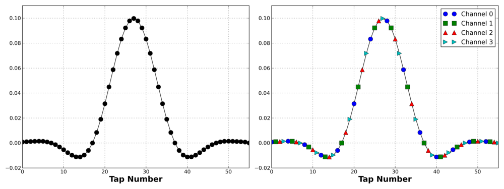
The code to generate this filter is:

lpf = filter.firdes.low_pass_2(1, 1, 0.05, 0.05, 60)

We use a 4 channel example here to make the visualization of the filter taps easy. But a more interesting channelization problem is do handle bigger sets of channels. Because it's easy and available, I'm using the FM broadcast band from 88 to 108 MHz. Each channel is 200 kHz wide, so there are 100 channels in the 20 MHz bandwidth. What would that filter look like?

Well, we can play around the parameters quite a bit to give us our desired performance. I'm going to intentionally introduce some slack to the filter with the knowledge rarely will we see two FM stations right next to each other in frequency. So I can go outside the channel bandwidth a bit so as to make a much cheaper filter. In this case, we use the parameters:

  • Type: FIR
  • Style: Low Pass
  • Window: Hann
  • Sample Rate: 20 MHz
  • Filter Gain: 1
  • End of Pass Band: 125 kHz
  • Start of Stop Band: 225 kHz
  • Stop Band Atten: 60 dB

The filter can be easily constructed and visualized using our gr_filter_design tool that comes installed with GNU Radio.

This builds a filter with 545 taps, which sounds like a lot. But we're constructing a filter that has a transition band of 100 kHz at a sample rate of 20 Msps, so what were we expecting? Luckily, however, the filterbank partitioning breaks this into 100 equal length filters, which means that each filter only has ceil(545/100) = 6 taps in it. Which sounds a lot better.

Channelizer

We can now use this filter two ways. First, let's use the PFB decimator (pfb_decimator_ccf) block. This, in its normal state, it just the normal fir_filter_ccf block of GNU Radio. But it has one extra parameter that allows us to take out the specified channel we are after whereas the normal FIR filter can only produce the baseband channel (channel 0 in our terms).

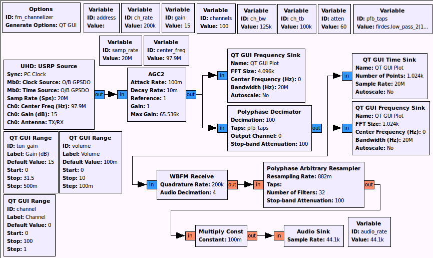
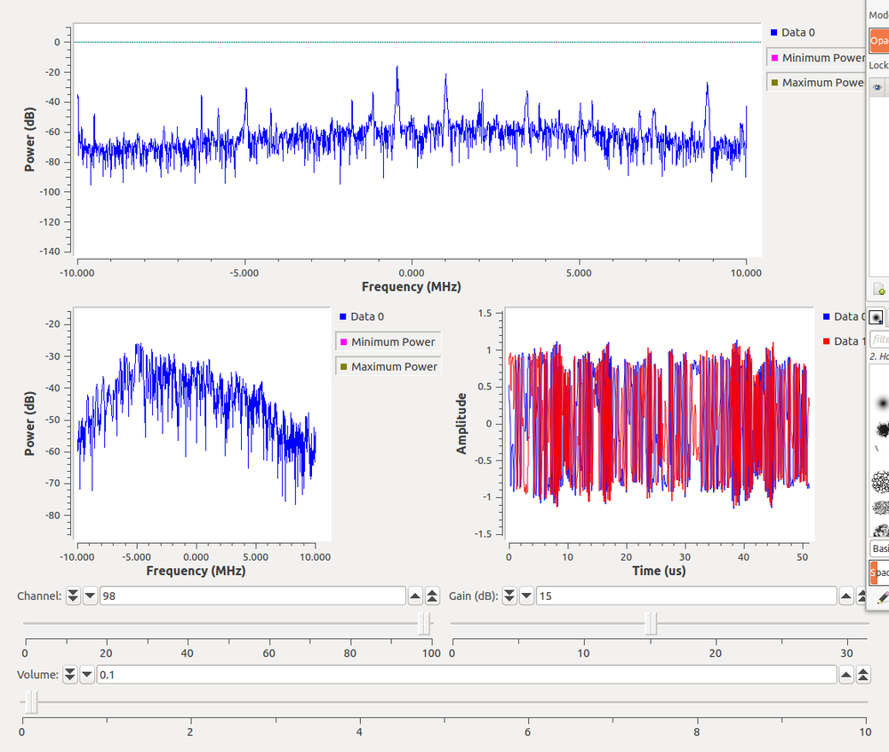
Using this GRC flowgraph, we take in samples from a radio. For this example, we have it set up as a UHD device and one that can specifically support 20 MHz of bandwidth. Mine on the desk in front of me is a USRP N210. We are then taking the wideband input channel and passing it to the PFB decimator with our given taps as shown above. The decimator's channel is actually a user-selected value during runtime, so we can very quickly move from one channel to another with the click of a mouse button. With this flowgraph, we can see the original full FM spectrum and the spectrum and time series of the selected channel.

And here's a resulting channelized FM station out of the flowgraph:


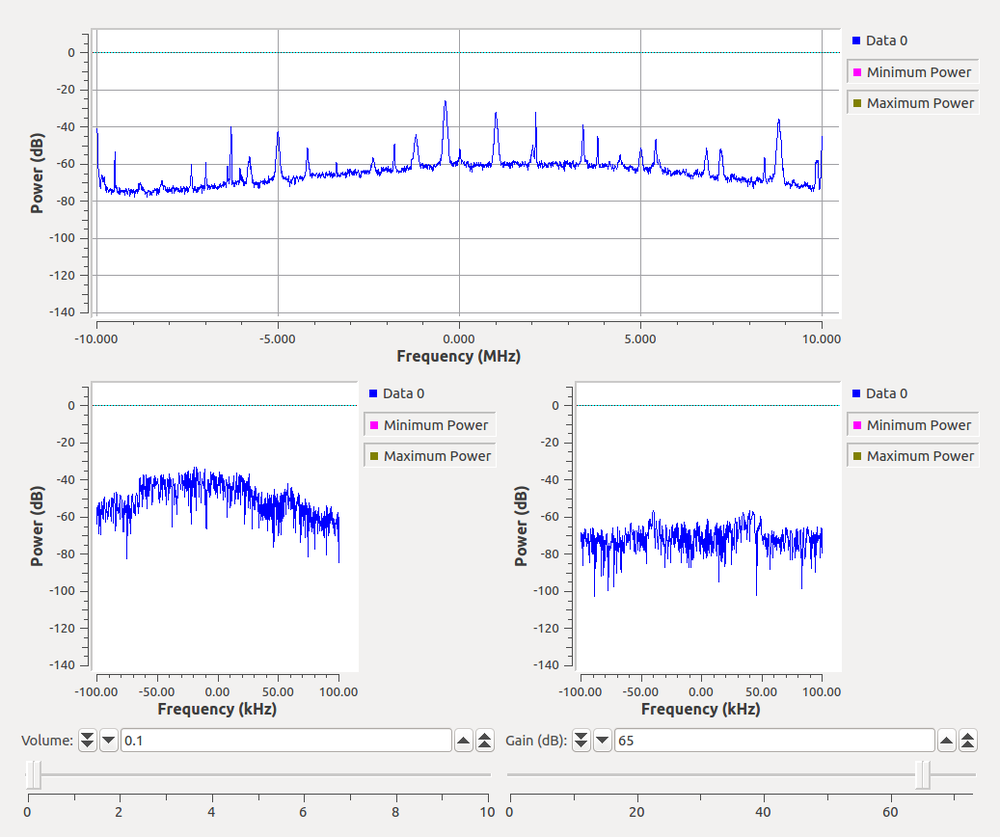
 We can also use this script that uses the channelizer to pull apart all channels at the same time.

Here, we're only showing two channels instead of all of them. But we could selectively pull out any channels we might want for the rest of the processing. The output of this looks like:

Just a word of caution. While the channelizer is fairly computationally efficient, we are still talking about working with 20 MHz, so you'll be using quite a bit of compute power, regardless. So don't be too surprised if you run into CPU limitations.

Synthesis Fitlerbanks

The synthesis filterbank is the reverse of the channelizer (also known as an analysis filterbank). It takes in multiple baseband channels and produces a single wideband spectrum. We'll use a very simple example to work through the basics of this. We'll just take four sine waves at different frequencies and synthesize them together.

First, we have to have some understanding about what the synthesizer does for us. In the digital domain, we can simply take in four signals and synthesize them on to four channels. But, what this turns in to is a situation where we are splitting channel 2 around the edge of the spectrum. Basically, the channel layout of the wideband spectrum looks like:

|  2  |    3    |    0    |    1    |  2  |

Channel 0 is the channel around DC (or 0 Hz), so because we are using an even number of channels, we split one channel around the fs/2 boundary. At complex baseband, this is fine, but we obviously wouldn't want to transmit this way. So the PFB synthesizer allows us to have more channels that we actually want to use. For this scenario, let's use six channels for the four signals. That way, we have the mapping:

|  3  |    4    |    5    |    0    |    1    |    2    |  3  |

Next we have the problem that if we insert four signals into the synthesizer, how do we tell it which output channels to use? By default, it will use channels 0 - 3, which leaves us with the same problem as before. The synthesis block has the ability to set the channel map, which changes the input stream to output channel accordingly. The map basically says that the channel on index x will output to channel channel_map[x]. The following figure might help explain it better.

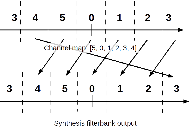
The flowgraph looks like the following. The original signals have frequencies of 10 kHz, -10 kHz, 20 kHz, and -20 kHz with a baseband sampling rate of 100 ksps. We use the channel map [5, 0, 1, 2, 3, 4] to left shift each channel once so that we avoid using channels 3 and 4.

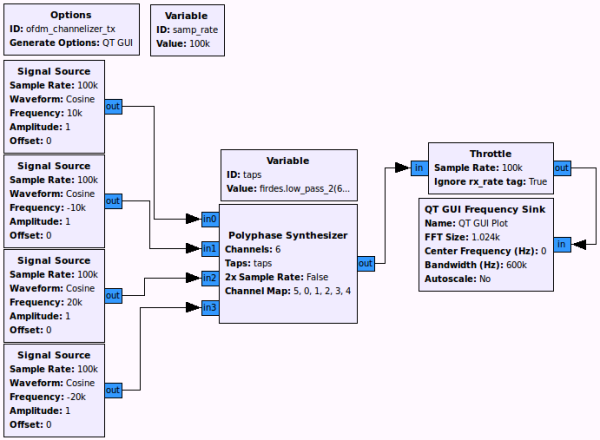
We expect the output to be at 600 ksps with sine tones at -90 kHz (the original 10 kHz), -10 kHz (originally -10 kHz), 120 kHz (originally 20 kHz), and 180 kHz (originally -20 kHz). The PFB synthesis filterbank's prototype filter was constructed using the following:

firdes.low_pass_2(6, 6*samp_rate, samp_rate/3.0, samp_rate/4.0, 60)

The filter, again, is designed at the high sampling rate, which is the output sampling rate of the synthesizer. The bandwidth is a bit less than the channel bandwidth with a bit of a roll-off. The output looks like:


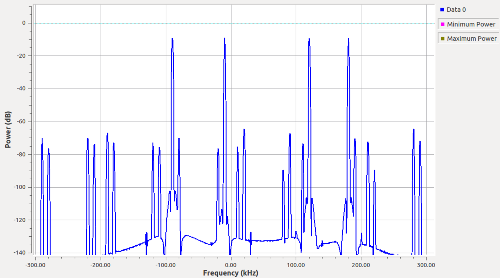
We can see the signals as the four peaks positioned exactly where we expected them to be. The other spikes throughout the spectrum are the result of synthesis process and aliasing of the channels, but notice that each is suppressed by about 60 dB or more from our peak signals. This is due to the fact that our out-of-band attenuation specification of the prototype filter was 60 dB. If more suppression is needed, we can make a more complex filter.

Reconstruction

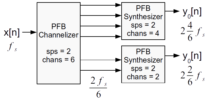
We'll end by going over the reconstruction filter. You can see in the paper the different steps of building up the filterbanks and how to analyze the reconstruction filters. The first case takes ten channels and fuses the results together while the second case takes six channels and recombines two and four of them as different outputs. You can download the Python scripts linked in the last sentence to look at how these behave. The following figure shows a diagram explaining the two output script.

The impulse scripts above are just good tools to understand how perfect our reconstruction is. The real trick to designing the reconstruction filters is to make sure that the end of the passband at -6 dB is at exactly the channel spacing and that the transition of the filter is set appropriately. Using the GNU Radio firdes, we can do this exactly and easily. The end of passband parameter we pass to our firdes filter designers specified where that -6 dB point will be, so we set that to half the channel's baseband sample rate. Using a Blackman-harris window with a stop band attenuation of 80 dB, the transition band should then be set to the baseband sample rate divided by 5. We're not quite sure, yet, why this number works, but Sylvain Munaut discovered this works universally for any sample rate while at our KIT hackfest last week. So given that fs is the baseband channel sampling rate, we can construct our filter as:

firdes.low_pass_2(1, M*fs, fs/2, fs/5, 80, firdes.WIN_BLACKMAN_HARRIS)

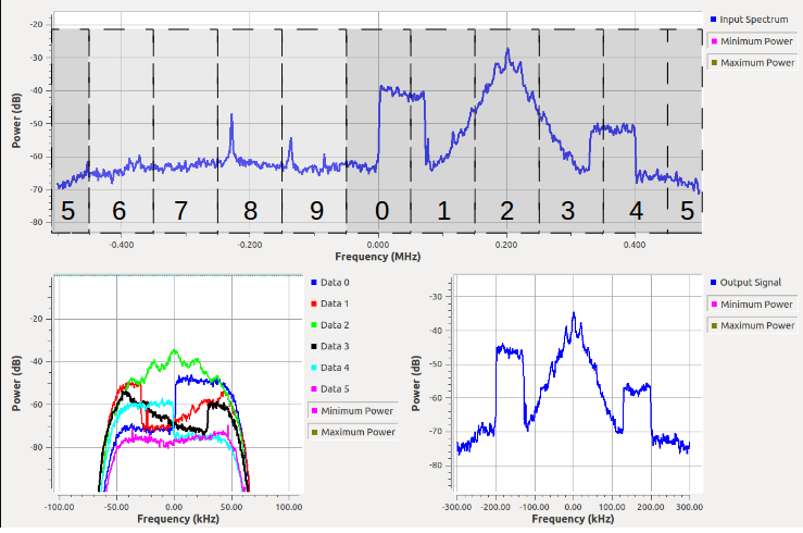
But the real result in the paper comes from taking an FM channel and splitting it into multiple channels and then reconstructing them again. We have the following flowgraph for this. You might have to change some settings on your UHD device to get it to work properly.

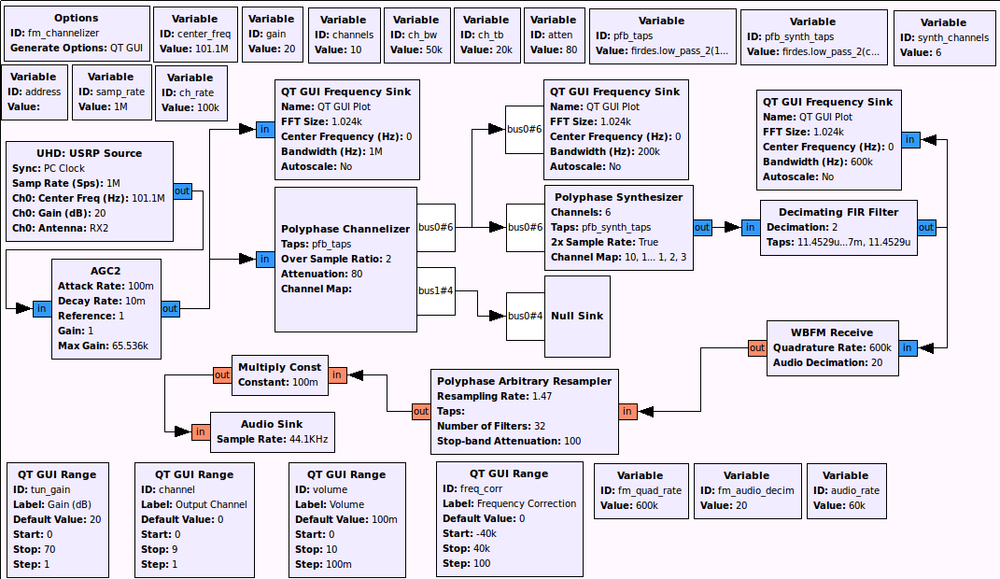
The result will look something like this, where the output of the synthesis filterbank is an FM signal centered at baseband that can then be demodulated like normal. This figure was edited to describe the channels, how the original signal was channelized, and which channels were synthesized to reconstruct it.

 I hope this walk-through of different uses of the channelizer and synthesis filterbanks helps make them a bit easier to use. Specifically, the prototype filter tends to be the hard part, but once the basics of it are understood, I expect that translating it to other needs shouldn't be terribly difficult for most people.

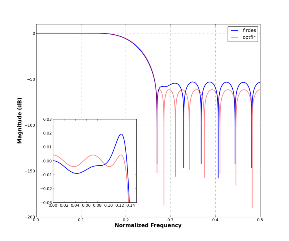
One thing that comes up with this study is our use of the firdes filter design tool, which uses windowed sinc functions. These tend not to be the most optimal, but I like them here because they are easy to design and control. Especially for our reconstruction filterbank work. Other filter design tools can be used, possibly more effectively, so there is nothing stopping anyone from designing their own filter however they like. The same principles of design and application will work.

Using QT Sinks

GNU Radio provides a couple of GUI interfaces using wxPython or QT. This example focuses just on the QT interface, gr-qtgui. Through a few small tweaks to an existing program, we can start to add QT sinks to the flow graph to start to visualize different signals, which can be especially useful when debugging and analyzing signals. The QT framework allows us to go even farther, though, and build entire applications in QT (using PyQT, for example). Also, the QT sink is written in C++ and wrapped into Python with SWIG, and so it should be possible to build C++-only applications using QT, although this hasn't been tested, yet.

In this example, though, we're just going to focus on inserting a QT sink into an existing flow graph to provide the basics of what is required to get a working GUI. We'll start with a simple application that adds two sine waves together with some additive Gaussian noise and outputs to a sink (I'm using a null sink here because we really don't care about the output until we add the GUI).

  1. #!/usr/bin/env python
  2. from gnuradio import gr
  3. class qt_top_block(gr.top_block):
  4.     def __init__(self):
  5.         gr.top_block.__init__(self)
  6.         self.src0 = gr.sig_source_c(Rs, gr.GR_SIN_WAVE, 0.01, 1)
  7.         self.src1 = gr.sig_source_c(Rs, gr.GR_SIN_WAVE, 0.10, 0.1)
  8.         self.noise = gr.noise_source_c(gr.GR_GAUSSIAN, 0.1)
  9.         self.add  = gr.add_cc()
  10.         self.snk  = gr.null_sink(gr.sizeof_gr_complex)
  11.         self.connect(self.src0, (self.add,0))
  12.         self.connect(self.src1, (self.add,1))
  13.         self.connect(self.noise, (self.add,2))
  14.         self.connect(self.add, self.snk)
  15. def main():
  16.     mytb = qt_top_block()
  17.     mytb.start()
  18.     mytb.wait()
  19. if __name__ == "__main__":
  20.     main()

This should look like a regular GNU Radio application right now. What we want to do, though, is add a QT sink. First, there's the boiler-plate stuff we have to insert into the project. We need to associate the class with the global qApp, which is done by adding a line in the constructor like: 

self.qapp = QtGui.QApplication(sys.argv)

Obviously, to access this information, we need to import QtGui and sys into the Python project. In the end, there are a few new modules we have to add. We'll get to those later.

The qApp let's us talk to the QT runtime engine, so we're going to have to make use of this later. For now, that's enough to make the qt_top_block class a QT application. Next, we need to build a QT sink. The prototype for the QT sink constructor looks like:

qtgui.sink_c(int fftsize, int wintype, double fc, double bandwidth, string name, bool plotfreq, bool plotwaterfall, bool plottime, bool plotconst, QWidget *parent);

 In this constructor, we can specify the size of the FFT points (e.g., 1024, 2048, etc.), the window type, which we can get from gr.firdes, and the center frequency and bandwidth to set up the axis. The "name" parameters is the title of the window that will appear in the title bar of the display. The next five arguments are all Boolean values that default to True and are used to determine whether or not to display a particular type of plot. The types of plots, in order, are the FFT, waterfall (spectrogram), 3D waterfall, time, and constellation plots. The final parameter is an optional parent, which defaults to None. When working a QT sink into a larger QT project, you can pass the parent information in this way.

Ok, so now we have a way to create a QT sink object. It acts like any other GNU Radio sink as far as the flow graph is concerned. We just connect a signal to it. Unfortunately, there's a bit of ugliness left to work through in order to expose the QT GUI -- we have to tell it to show itself. This is done by getting a QWidget instance of the object in Python and calling the show() function on this. 

Putting all of this knowledge together leads to the code below (which you can download here: qt_basics.py). There are a few new lines that I will explain afterwards.

  1. #!/usr/bin/env python
  2. from gnuradio import gr
  3. from gnuradio.qtgui import qtgui
  4. from PyQt4 import QtGui
  5. import sys, sip
  6. class qt_top_block(gr.top_block):
  7.     def __init__(self):
  8.         gr.top_block.__init__(self)
  9.         Rs = 1
  10.         fftsize = 2048
  11.         self.qapp = QtGui.QApplication(sys.argv)
  12.         self.src0 = gr.sig_source_c(Rs, gr.GR_SIN_WAVE, 0.01, 1)
  13.         self.src1 = gr.sig_source_c(Rs, gr.GR_SIN_WAVE, 0.10, 0.1)
  14.         self.noise = gr.noise_source_c(gr.GR_GAUSSIAN, 0.1)
  15.         self.add  = gr.add_cc()
  16.         self.thr  = gr.throttle(gr.sizeof_gr_complex, 10e5)
  17.         self.snk  = gr.null_sink(gr.sizeof_gr_complex)
  18.         self.qtsnk  = qtgui.sink_c(fftsize, gr.firdes.WIN_BLACKMAN_hARRIS,
  19.                                    0, Rs,
  20.                                    "Complex Signal Example",
  21.                                    True, True, False, True, False)
  22.         self.connect(self.src0, (self.add,0))
  23.         self.connect(self.src1, (self.add,1))
  24.         self.connect(self.noise, (self.add,2))
  25.         self.connect(self.add, self.snk)
  26.         self.connect(self.add, self.thr, self.qtsnk)
  27.         pyWin = sip.wrapinstance(self.qtsnk.pyqwidget(), QtGui.QWidget)
  28.         pyWin.show()
  29. def main():
  30.     mytb = qt_top_block()
  31.     mytb.start()
  32.     mytb.qapp.exec_()
  33.     mytb.stop()
  34. if __name__ == "__main__":
  35.     main()

Now, instead of just importing the gr namespace, lines 3-5 import the GNU Radio qtgui module, QtGui from PyQT, and sys and sip. In line 11, we get our reference to the qApp, which takes in a set of arguments that we get from sys.argv. We tend to ignore this, though, although advanced users can manipulate the system through this interface. Lines 18 - 21 call the qtgui constructor for a complex sink (sink_c). Following the prototype above, we create a sink where the FFT size is initially 2048, we use a Blackman-harris window, set the center frequency to 0, and the bandwidth is just 1.  We then give the window a title, "Complex Signal Example," and turn on the FFT, waterfall, and time plots.

Line 26 connects the sink to the graph, so the output of the adder will be displayed. Notice that I also put the signal through a throttle. I did this to control the speed of the graph. Without anything external to clock the samples such as an audio device or a USRP, the graph would simply run as fast as possible. The gr_throttle allows us to set a simulated sample rate so that when we graph it, we can actually see what's going on. Try removing the throttle from the graph, but be prepared for the application to take over your computer :)

Lines 27 and 28 are what I meant about getting a QWidget instance and calling the show() function. Using sip, which is a PyQT program for getting QT stuff into Python, allows us to get a Python version of a QWidget so that we can actually call the show() function on a widget. There doesn't seem to be a good way to do this otherwise, so I exposed the pyqwidget function in the qtgui sink classes. The problem comes down to who owns the qApp and the widgets in order to display them. This is uglier than I wanted it, but it's just an odd two lines of code, which was better than some alternatives that were tossed around...

The final change required is to call the qApp's executor function. This is a blocking loop, so we can first start the flow graph as a non-blocking call with mytb.start(). Instead of calling mytb.wait() like we originally did, we now let the QT framework lifecycle take over in line 32 with mytb.qapp.exec_(). Make sure to call mytb.stop() to properly shut down the flow graph and delete the objects in the proper order.

When you run this program, you will see a display that looks like the following. The display starts by showing the Frequency plot (if it's activated, of course).

 The next tab shows the waterfall display (or spectrogram) that starts at the bottom of the screen and moves up. This image was captured after a few seconds had passed. I also hit the "Auto Scale" button in order to set the dynamic range of the color bar to best represent the range of the signal (in this case from 0 dB to about -64 dB).

The last tab in this case shows us the time waveform, showing a trace for both the real and imaginary parts of the signal.

 Notice that the display has a few different controls. For one, while we set the initial FFT size to 2048, this can be changed in real-time by clicking the "FFT Size" drop-down box and selecting from a handful of preset sizes (all powers of 2). This will adjust the resolution in the frequency and waterfall plots and will increase the number of samples displayed in the time domain plot.

We can also tell the display to show the frequency domain relative to the RF frequencies. This check box really just uses the fc argument we passed to the constructor to reset the x-axis of the frequency and waterfall plots.

Another drop-down box exposed for us to change in the FFT window. While we initialized with the Blackman-harris window, this gives us the option of whatever windows are available in GNU Radio, which currently includes Hamming, Hann, Blackman, rectangular, Kaiser, and Blackman-harris.

The frequency domain plot has a few of its own interfaces to work with. First, you can set the min and max holds and reset them as you want to. The Average box tells the GUI to average a certain number of plots, which can help smooth out noise. Also, there are a few lines drawn on this display, including a line (green) showing the value of the maximum signal in the current display as well as a line (cyan) of the average noise.

The waterfall plot also has a few things to play with. As I already mentioned, you can auto scale the intensity bar range, or you can manually adjust using the two wheels. The top wheel sets the upper bound of the intensity plot while the bottom wheel sets the lower bound. Furthermore, you can change the color scheme with the "Intensity Display" drop-down box, which includes a "User Defined" selection that lets the user set the upper and lower colors for the plots and then interpolates between them.

One final note about the plots is that each of the figures allows you to position the cursor anywhere in the plot and it will tell you the current values. By left-clicking with the mouse and dragging a box, you can zoom in to any region, too. You can zoom in about 10 times. A right-click will back up a single zoom step.

So that's the basics of how to incorporate a QT gui into a flow graph and how to use the figures.

Basic Filtering

This example shows the basics of how to use a filter in GNU Radio. First, we have to generate a set of filter taps, which can be a vector of either real complex values. While you are welcome to generate the taps any way you would like, GNU Radio provides a few generating functions to make this easier.

Basic Filters

The first example shows the use of the "firdes" utility, which is used to generate windowed FIR filters. Here, I am creating a simple low pass filter (LPF). There are generally two versions of each type of filter. Those with the "_2" extension provide a means of specifying the out-of-band (or stopband) attenuation (in dB). Generally, you want to use this version as it costs you almost nothing but gives you an extra parameter to control.

Example code: filter_basics.py

In this example, we create a low pass filter using the function:

    lpf_taps = filter.firdes.low_pass_2(1, 1, 0.2, 0.1, 60)

We are specifying, in order, the filter gain, sample rate, center of the transition band, the transition band width, and the stopband attenuation (in dB). The center of the transition band specifies the point where the rolloff is 6 dB down from the passband. This value and the transition band are set relative to the sample rate. Since the sample rate here is set to 1.0, we must also specify normalized bandwidths. We can also use a real sample rate here and scale the widths appropriately in terms of Hz.

The filter_basics.py example shows the use of two filters: filter.fir_filter_ccc and filter.fft_filter_ccc. These take the same arguments and both filter a signal with the same filter taps. The difference is in how they do it. The version with "fir_" performs a straight-forward implementation of an FIR filter by performing the convolution in time. The "fft_" version, however, performs the fast-convolution, which means that it takes an FFT and performs the convolution as a multiplication in the frequency domain. The results are then passed through an IFFT to get the samples back into the time domain. 

For small filters, which is somewhere around 30-taps and fewer, the FIR filter version performs faster. However, the fast-convolution takes advantage of faster multiplies and the inexpensive FFT and IFFT operations. For larger filters (greater than 30), these operations perform better than the FIR filter.

The figure below shows the output of filtering a noise signal with both an FIR and FFT version of the same filter. While this does not show off the difference in speed, it shows that the output is the same. In time, they look almost identical. In the frequency domain, we can see a slight difference due to numerical precision that is negligable.

To compare the processing time of the different filers, you can use the filter_timing.py file. It takes a few minutes to run as is. The variables N, start, stop, and step can be easily changed to examine different aspects of the behavior. Looking at the times for 1024 taps (sampled every 2 taps) produces the following image. This was on an Intel i7-2620M CPU with AVX enabled in VOLK. The FIR filter climbs nearly linearly, though the step-wise pattern is likely related to something in the VOLK vectorized processing. However, the FFT filter is nearly flat over all filter sizes. It also shows that on this processor, the crossover point is a very small number of taps; in fact, it's close to 1.

Windowed and Parks-McClellen Filters

The second example shows the use of a second GNU Radio filter design utility called "optfir" module, also a part of the "filter" module. However, the optfir module is built entirely in Python while firdes is written in C++. This filter designer uses the Parks-McClellen algorithm for designing filters. Unlike the firdes windowed filters, this utility gives you another degree of freedom when designing filters: the passband ripple (in dB).

You have to watch out for this utility, though, especially if you are comfortable with using firdes. In the firdes utility, you specify the center of the transition band, which is 0.5 in linear amplitude or -6 dB in log power scale. You also specify the transition band, which is the width from the cutoff to the stopband. On the other hand, in the optfir utility, you will specify the end of the passband(s) and start of the stopband(s) (plural if you are designing bandpass filters). The end of the passband is the point when the filter roll-off begins, not the 3-dB or 6-dB point, and the start of the stopband is where the first null occurs. Keep in mind, though, that these values are going to be approximate since the Parks-McClellen algorithm is an optimization technique that attempts to fit a filter to the desired specs.

In the following example, I tried to design a LPF with both the firdes and optfir filters that were approximately the same filter, by which I mean having the same passband and stopband. What is different is that the specified passband ripple from optfir gives me a much lower ripple for the same number of filter taps (27 in this case). If we specified a ripple of, say 0.03 dB, we can reduce the filter size a bit farther. The point here being that for approximately equivalent filters, you are generally going to get a smaller filter using the Parks-McClellen.

We create the taps with the following function calls.

    firdes_taps = filter.firdes.low_pass_2(1, 1, 0.2, 0.1, 60)

    optfir_taps = filter.optfir.low_pass(1, 1, 0.13, 0.2675, 0.01, 60)

Filter example with optfir: filter_optfir.py

A few good explanations:

Julius O. Smith: 

http://www.dsprelated.com/dspbooks/sasp/FIR_Digital_Filter_Design.html

http://www.dsprelated.com/dspbooks/sasp/Window_Method.html


Other:

http://www.dspguru.com/dsp/faqs/fir/design


Simple Signals

I just wanted to get a simple application programmed up and available for people to see the basics of GNU Radio. In this equivalent of a "hello world," I'm simply creating a couple of signal sources and outputting them to a vector sink. To display the results, I'm using the Python package Matplotlib, which can be easily installed in almost any operating system.

The output is displayed below showing the resulting signal in both time and frequency.

Code: simple.py