Blog

To Use or Not to Use FFT Filters

I've talked in various presentations about the merits of fast convolution, which we implement in GNU Radio as the fft_filter. When you have enough taps in your filter, and this is architecture dependent, it is computationally cheaper to use the fft_filter over the normal fir_filters. The cross-over point tends to be somewhere between 10 and 30 taps depending on your machine. On my AVX-enabled system, it's down around 10 taps.

However, Sylvain Munaut pointed out decreasing performance of the FFT filters over normal FIR filters when decimating a high rates. The cause was pretty obvious. In the FIR filter, we use a polyphase implementation where we downsample the input before filtering. However, in the FFT filter's overlap-and-save algorithm, we filter the input first and then downsample on the output, which means we're always running the FFT filter at full rate regardless of how much or little data we're actually getting out of it.

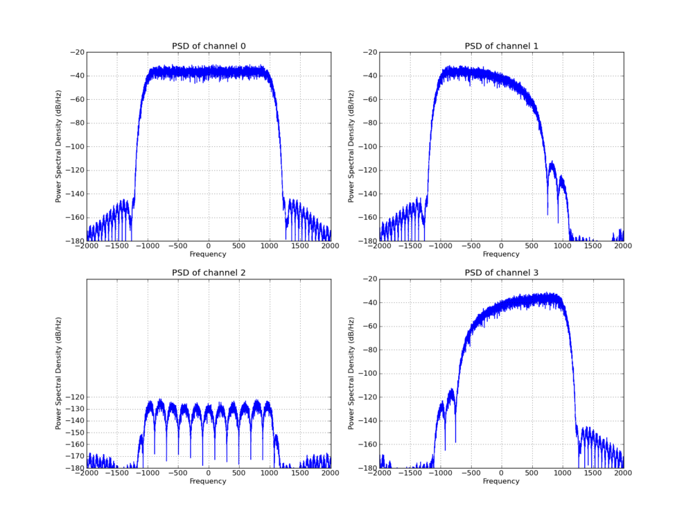
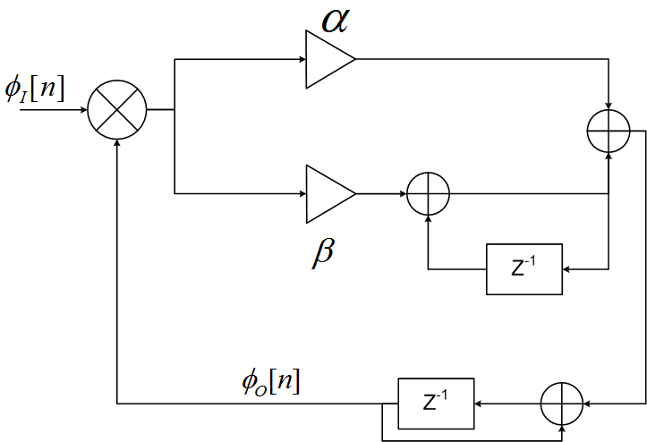
GNU Radio also has a pfb_decimator block that works as a down-sampling filter and also does channel selection. Like the FIR filter, this uses the concept of polyphase filtering and has the same efficiencies from that perspective. The difference is that the FIR filter will only give you the baseband channel out while this PFB filter allows us to select any one of the Nyquist zone channels to extract. It does so by multiplying each arm of the filterbank by a complex exponential that constructively sums all of the aliases from our desired channel together while destructively cancelling the rest.

After the discussion about the FIR vs. FFT implementation, I went into the guts of the PFB decimating filter to work on two things. First, the internal filters in the filterbank could be done using either normal FIR filter kernels or FFT filter kernels. Likewise, the complex exponential rotation can be realized by simply multiplying each channel with a complex number and summing the results, or it could be accomplished using an FFT. I wanted to know which implementations were better.

Typically with these things, like the cross-over point in the number of taps between a FIR and FFT filter, there are going to be certain situations where different methods perform better. So I outfitted the PFB decimating filter with the ability to select which fitler and which rotation structures to use. You pass these in as flags to the constructor of the block as:

  • False, False: FIR filters with complex exponential rotation
  • True, False: FIR filters with the FFT rotator
  • False, True: FFT filters with the exponential rotator
  • True, True: FFT filters with the FFT rotator

This means we get to pick the best combination of methods depending on whatever influences we might have on how each performs. Typically, given an architecture, we'll have to play with this to understand the trade-offs based on the amount of decimation and size of the filters.

I created a script that uses our Performance Counters to give us the total time spent in the work function of each of these filters given the same input data and taps. It runs through a large number of situations for different number of channels (or decimation) and different number of taps per channel (the total filter size is really the taps len times the number of channels). Here I'll show just a handful of results to give an idea what the trade-off space looks like for the given processor I tested on (Intel i7-2620M @ 2.7 GHz, dual core with hyper threading; 8 GB DDR3 RAM). This used GNU Radio 3.7.3 (not released, yet) with GCC 4.8.1 using the build type RelWithDebInfo (release mode for full optimization that also includes debug symbols).

Here are a few select graphs from the data I collected for various numbers of channels and filter sizes. Note that the FFT filter is not always represented. For some reason that I haven't nailed down, yet, the timing information for the FFT filters was bogus for large filters, so I removed it entirely. Yet, I was able to independently test the FFT filters for different situations like those here and they performed fine; not sure why the timing was failing in these tests.

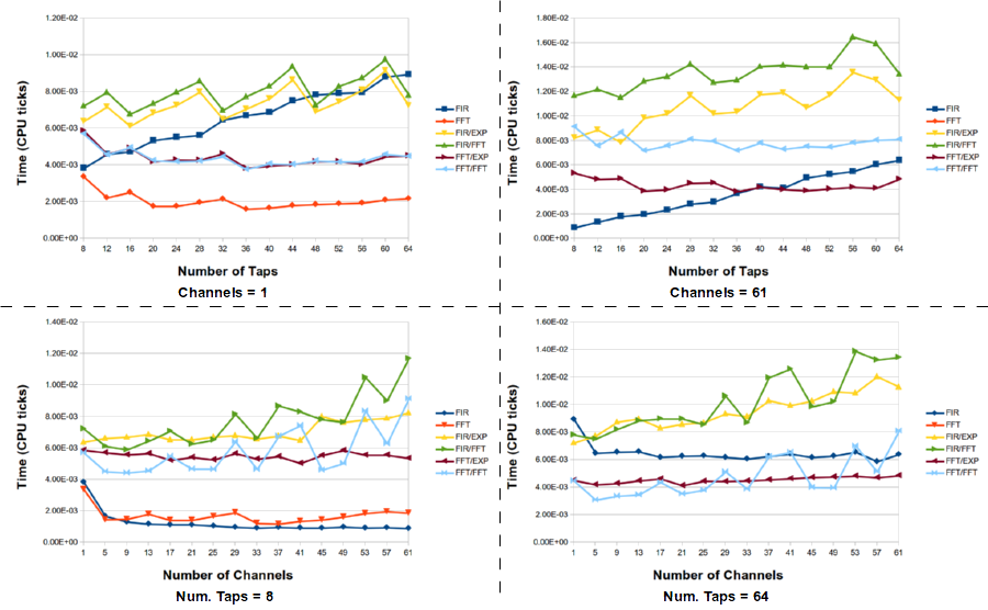
We see that the FIR filters and FFT filters almost always win out, but they are doing far fewer operations. The PFB decimator is going through the rotation stage, so of course it will never be as fast as the normal FIR filter. But within the space of the PFB decimating filters, we see that generally the FFT filter version is better while the selection between the exponential rotator and FFT rotator is not as clear-cut. Sometimes one is better than the other, which I am assuming is due to different performance levels of the FFT for a given number of channels. You can see the full data set here in OpenOffice format.

Filtering and Channelizing

A second script looks at a more interesting scenario where the PFB decimator might be useful over the FIR filter. Here, instead of just taking the baseband channel, we use the ability of the PFB decimator to select any given channel. To duplicate this result, the input to the FIR filter must first be shifted in frequency to baseband the correct channel and then filtered. To do this, we add a signal generator and complex multiply block to handle the frequency shift, so the resulting time value displayed here is the sum of the time spent in each of those blocks. The same is true for the FFT filters.

Finally, we add another block to the experiment. We have a freq_xlating_fir_filter that does the frequency translation, filtering, and decimation all in one block. So we can compare all these methods to see how each stacks up.

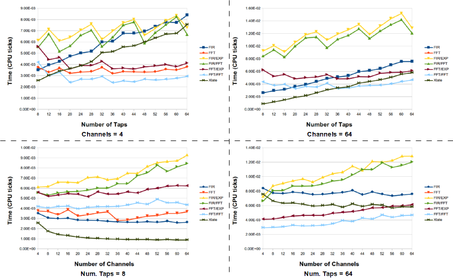
What this tells us is that the standard method of down shifting a signal and filtering it is not the optimal choice. However, the best selection of filter technique really depends on the number of channels (e.g., the decimation factor) and the number of taps in the filter. For large channels and taps, the FFT/FFT version of the PFB decimating filter is the best here, but there are times when the frequency xlating filter is really the best choice. Here is the full data set for the channelizing experiments.

One question that came to mind after collecting the data and looking at it is what optimizations FFTW might have in it. I know it does a lot of SIMD optimization, but I also remember a time when the default binary install (via Ubuntu apt-get) did not take advantage of AVX processors. Instead, I would have to recompile FFTW with AVX turned on, which might also make a difference since many of the blocks in GNU Radio use VOLK for SIMD optimization, including AVX that my processor supports. That might change things somewhat. But the important thing to look at here are not absolute numbers but general trends and trying to get a feeling for what's the best for your given scenario and hardware. Because these can change, I provided the scripts in this post so that anyone else can use them to experiment with, too.


Some Really Cool DSP

I finally took the time to really understand the polyphase synthesis filterbank and how to use it to reconstruct previously channelized signals. Once again, I looked to fred harris' work on the subject and have cracked it. The keys are in creating an M-to-2fs PFB channelizer, a 2-to-Pn PFB synthesizer, and perfect reconstruction filters (-6 dB at the edge of the passband).

I plan on writing up a more thurough look into this, and all of the code to do the proper synthesis filter will be going into GNU Radio soon, but for now, some pretty pictures.

First, we start off with a QPSK signal with very little noise:

Here, I split the signal up into 4 equally spaced channels. Channel 0 is around DC (0 Hz) and goes from -1000 - 1000 Hz, channel 1 is from 1000 - 3000 Hz, and channel 3 is from -3000 to -1000 Hz. Now, channel 2 actually spans from 3000 - 4000 and then wraps around to go from -4000 to -3000 Hz. These have a 1000 Hz bandwidth but are sampled at 2 samps/symbol so the channel sample rate is 2000 Hz.

I then go through the 2-to-Pn synthesizer where Pn is actually 8. This synthesis filter takes 4 channels in and produces four channels but at twice the sampling rate, so we now have a signal that is the original signal but sampled at twice the orignal rate. Notice also that it's offset by a bit in frequency in the PSD. That's a result of my plotting that I don't feel like correcting (it's related to the reason why channel 2 spans the edge of the positive and negative spectrum). Obviously, the constellation is not rotating, so we're ok.

Notice also that this signal was first split up, filtered, and then put back together again. Perfectly. That constellation should be enough proof of that. This has some huge implications to what we can do with this concept once I generalize it. This was a simple demonstration to get the algorithm and math correct, but now we can have some serious fun!

For those of you into such things, this is the filter I used for this example:

I generated it using GNU Radio firdes.low_pass_2 filter generator with these parameters:

  • Gain = 1
  • Sample Rate = 8000 Hz
  • Bandwidth = 1000 Hz
  • Transition bandwidth = 200 Hz
  • Attenuation = 80 dB
  • Window: Blackman-harris


SNR Estimators

In GNU Radio, we have been slowly evolving our digital communications capabilities. One thing that becomes quickly and painfully obvious to anyone doing real over-the-air communications with digital modulations is that the modulators and demodulators are the easy part. It's the synchronization that's the hard part and where most of your work as a designer goes.

Generally speaking, synchronization means three (maybe four) things: frequency, timing, and phase. The fourth is automatic gain control (AGC). While AGC isn't really "synchronization," it follows similar principles of an adaptive loop. Different modulation schemes have different methods for AGC and synchronization. These tend to fall into categories of narrowband, wideband (and then ultrawideband), and OFDM, but we can easily dispense with these categories and go in depth into differences within them, too. For instance, narrowband PSK and FSK systems have pretty widely different requirements out of a receiver for demodulation and the appropriate synchronization algorithms reflect this.

But this post is about SNR estimation. The reason to talk about synchronization here it twofold. First, like synchronizers, SNR estimation techniques can vary widely depending on the modulation scheme being used. Second, most synchronization schemes like to be reactive to changes in SNR. You can often find different algorithms that work well in low SNR cases but not high, or they are too costly to perform in high SNR where the signal quality allows you to use something simpler and/or more accurate. Take for example an equalizer. The constant modulus equalizer is great for PSK signals, but we know that an LMS decision-directed equalizer works better. But a decision-directed equalizer only works in cases where the SNR is large enough that the majority of samples are correct. So we often start with a blind CMA for acquisition purposes and then move to a decision-directed approach once we've properly locked on to the signal.

We've been meaning to add SNR estimators to GNU Radio for some time, now, and I finally developed enough of an itch to start doing it. But as I said, each modulation could use a different equalizer, and there are various equalizers designed for this modulation in that channel or that modulation in such and such channel. If you have access to IEEExplore, a simple search for "snr estimator" produces 1,279 results. Now, I know that's nothing to a Google search, but twelve hundred scholarly (we hope) articles on a topic is a lot to get through, and you will quickly see that there are finely-tuned estimators for different modulations and channels.

What I did was give us a start into this area. I took a handful of the most generic, computationally realistic estimators that I could find for PSK signals and implemented them. I'll give a shout out here to Normon Beaulieu, who has written a lot in this field. I've found that a lot of his work in SNR estimators to be accessible and useful, and he presents his work in ways that can be easily translated into actual, working code.

I also took the tack of looking for estimators that worked in AWGN channels. Now, if you've ever heard me speak on the subject of communications education or research, you've probably heard me scoff at anyone who develops a system under simulated AWGN conditions. In the case of an SNR estimator, though, I thought about this and had to come to the conclusion that the only way to handle this is to have an estimator that you can plug in variables for your channel model, which of course assumes that you have or can estimate these parameters. So in the end, I followed Beaulieu's lead in at least one of this papers and took algorithms that could be both simplified and tested by assuming AWGN conditions. I did, however, provide one of these algorithms (what I refer to as the M2M4 algorithm) in a way that allows a user to specify parameters to better fit a non-AWGN channel and non-PSK signals. Using the AWGN-based algorithms with this other version of the M2M4 seemed like a good compromise for being computable without more information but at least providing a tip of my hat to the issue of non-AWGN channels. If nothing else, these estimators should give us a ballpark estimate.

I also specifically developed these estimators based on a parent class that would easily allow us to add more estimators as they are developed. Right now, the parent class is specifically for MPSK, but we can add other estimator parent classes for other modulations; maybe have them all inherit from a single class in the end -- this is fine, since the inheritance would really be hidden from the end user. The class itself is in the gr-digital component and called digital_impl_mpsk_snr_est. It's constructor is simply:

digital_impl_mpsk_snr_est(double alpha);

Where the parameter alpha is the value used in a running average as every estimator I've seen is based on expected values of a time series, which we estimate with the running average. This value defaults to 0.001 and should be kept small.

I have created four estimators that inherit from this block. These are named the "simple," "skew," "M2M4," and "SVR" estimators. The last two come from [1]. The "skew" estimator uses a skewness measure that was developed in conversation with fred harris. The simple estimator is probably written up and documented somewhere, but it's the typical measurement based on the mean and variance of the constellation cloud.  I've tried to document these as best as possible in the header files themselves, so I'll refer you to the Doxygen documentation for details (note that as of the writing of this blog post, these estimators are only in the Git repository but will be available starting in the 3.5.1 release). The "SNR estimators"  group in the Doxygen manual can be used to find all of the available estimators and details about how to use them.

In particular, the M2M4 and SVR methods were developed around fading channels and both use the kurtosis of the modulation signal (k_a) and kurtosis of the channel (k_w) in their calculations. This is great if these values are know or can be estimated. In the case of the M2M4 algorithm, I provide a version of it, called the digital_impl_snr_est_m2m4, as an example of a non-PSK and non-AWGN method; right now, this block is unavailable through any actual GNU Radio block. It's untested and unverified, but I wanted it there for reference and hopefully to use later.


SNR Use in Demodulation

The main intent of having an SNR estimator block is to enable the use of SNR information by other blocks. As such, there are two GNU Radio blocks that are defined for doing this in different ways. First off, let's say that the SNR estimation is done after timing recovery (see harris' paper "Let’s Assume the System is Synchronized", which is unfortunately fairly costly but worth it if you can get a copy). So in GNU Radio terms, this means that the SNR is estimated down stream of most of the synchronization blocks. While I would like to just pass a tag along with the SNR information, that does won't work for every block, like the frequency recovery, AGC, and timing recovery loops that come before. Instead, we will have to pass them a message with this information. However, some blocks exist downstream that want this info, too, like the channel equalizer.

To accommodate both possible uses, I created two blocks. The digital_mpsk_snr_est_cc block is a flowgraph with a single input and single output port, so it's meant to go inline in a flowgraph. This block produces tags with the SNR every N samples, where N is set by the user (the second arg in the constructor and through the set_tag_nsamples(int N) function). The downstream blocks can then look for the tag with the key "snr" and pull out this information when they need it. The value of N defaults to 10,000 as an arbitrary, fairly large number. You'll want to set this depending on the speed you expect the SNR conditions to change.

The second block is a probe, which is GR speak for a sink. It's called digital_probe_mpsk_snr_est_c and only takes a single complex input stream. Right now, it just acts as a sink where the application running the flow graph can query the SNR by calling the "snr()" function on this block (the same is true for the digital_mpsk_snr_est_cc block, too). However, this block uses a similar constructor in that you set a value N for the number of samples between messages. In this case, instead of sending a tag down stream, it will send a message every N samples. The problem with this is that our message passing system isn't really advanced or easy enough to use to set this up properly. Recent work by Josh Blum might fix this, though.

Eventually, though, we hope to be able to create flow graphs where the SNR estimation is passed around to other blocks to allow them to adjust their behavior. In the case I'm interested in right now, I'd like to pass this info to the frequency lock loop to stop it if the SNR falls below a certain level so that it doesn't walk away when there is no signal to acquire.


[1]  D. R. Pauluzzi and N. C. Beaulieu, "A comparison of SNR estimation techniques for the AWGN channel," IEEE Trans. Communications, Vol. 48, No. 10, pp. 1681-1691, 2000.


Control Loop Gain Values

I have recently been working on updating our digital modulation capabilities in GNU Radio. This has involved making a gr-digital namespace, moving all relevant digital modulation work over, and going through and fixing up a number of the algorithms. One issue in particular that I have been working on is the concept of the loop gains in all of our control loops. You will find in any control loop we have, like in the clock recovery, Costas loop, constellation receiver, FLL and PLL blocks, that the control loop has two gains, alpha and beta. These are used in the following ways:

freq = freq + beta * error

phase = phase  + freq + alpha * error

When creating any of these blocks, we have to specify both alpha and beta. But what should these values be? What relationship do they have to each other, or, indeed, the physical properties of the control loop? Well, that's not easy to understand or explain, and because of this, it's not the right way to build these algorithms.

A better way is to convert these gains into a damping factor and loop bandwidth, which gives us a bit more intuition as to what's going on and makes them easier to set. So I have been switching over to using these concepts instead of alpha and beta. The loop equations are the same, and so we have to derive alpha and beta from these two new concepts. This is done in the following way where damp is the damping factor and bw is the loop bandwidth:

alpha = (4 * damp * bw) / (1 + 2 * damp * bw + bw * bw)

beta = (4 * bw * bw) / (1 + 2 * damp * bw + bw * bw)

So now we just have to know what damping factor and bandwidth we require from our loops. Of course, right now it seems like we've just translated from one set of unknowns to another set of unknowns. But at least we can better explain this new set. In fact, we're going to break it down so that we only specify one of those numbers.

In control systems, the damping factor specifies the oscillation of the loop, whether it's under, over, or critically damped. In a normalized system, a damping factor of 0.707 (or the sqrt(2)/2) is a critically damped system. This is a good approximation for most systems, so we can just set it and forget about it. 

So now, we just have to set a loop bandwidth. This is a bit more difficult, but as a rule, this value should be somewhere around (2pi/100) to (2pi/200), so we can work around there. If we're trying to optimize the behavior of our system, it's now a hell of a lot easier to work with a single value instead of two.

Just to be complete about the whole thing, though, as I have been reworking all of these blocks, I have also been adding set and get functions for every value. So while the constructor only needs us to give it the loop bandwidth, we can also change the damping factor if there's a particular need to do so. We can also individually change alpha and beta, still, if really want to.