Blog

QT GUI Widgets with Message Passing

 Just today, I issued a Pull Request for a new feature in GNU Radio. This adds a new form of what we already called the QT GUI Entry widget. That widget provides a simple QLineEdit box where we type in values, they get stored as a Python variable, and we pass these variables around like normal GRC variables. When running, updates to the entry box are propagated to anything using that variable in the flowgraph.

We're trying to move beyond this world where everything is in a Python file that's assumed to be completely local. Instead, we want to move to a world where we can use the message passing architecture to manage data and settings. So when we have a message interface to a block, we might want to post data or update a value through that message interface from a UI somehow. This leads us to the possibility that the UI is a separate window, application, or even machine from the running flowgraph. We have already made strides in this direction by adding the postMessage interface to ControlPort, which I spoke about in the last post on New Way of Using ContorlPort. However, ControlPort can take some time to set up the application, craft the UI, and make a working product. Aside from that method, we wanted to have easy ways within GRC to build applications that allow us to pass and manage messages easily. Hence the new QTGUI Message Edit Box (qtgui_edit_box_msg).


This is an flowgraph example that now comes with GNU Radio's gr-qtgui (test_qtgui_msg.grc). This shows the use of three of the new message edit boxes. In the upper part of the graph, we have the edit box controlling the center frequency of a Waterfall and Frequency Sink. These sinks can take in a message that's a PMT pair in the form ( "freq" <float frequency> ). So the edit box has a setting called Pair that sets this up to handle the PMT pair messages. It's actually the default since we'll be using the key:value pair concept a lot to manage message control interfaces. When the edit box is updated and we press enter, it publishes a message and the two GUI sinks are subscribed to them, so they get the message, parse it, and update their center frequency values accordingly.

Now the flip side of this is that the edit boxes also have an input message port. This allows us to programmatically set the value inside the box. The two GUI sinks have the ability to have a user adjust their center frequency. When a user double-clicks on a frequency in the plot, the block sets that value as the center frequency and then publishes a message (in the same key:value pair where key="freq"). This means that not only is the widget we just double-clicked updated, anything listening for that message is updated. So the edit box is kept in sync with the change in the GUI. Now, when the new data received is different than what was in that edit box to begin with, the box re-emits that message. So now, say we double-clicked on the Frequency Sink near the 10 kHz frequency line. That message is propagated not only to the edit box, but the message also gets sent from that box through to the waterfall sink. Now all of the widgets are kept in sync. And because the re-posting of the message only happens when a change occurs, we prevent continuous loops. Here's the output after the double-clicking:

Both GUI display widgets have the same center frequency, and that value is also shown in the Frequency edit box above. Because it's using the pair concept, we have two boxes, the left for the key and right for the value.

This example has two other edit boxes that show up at the bottom of the GUI. This is to allow us to easily test other properties and data types. They are connected in a loop, so when one is changed, the other immediately follows. Note here that we are not using the pair concept but that the data type is complex. To make it easy on us, we use a Boost lexical_cast, which means we use the format "(a,b)" for the real and imaginary parts. All of this, by the way, is explained in the blocks'd documentation.

Now, we have the ability to pass messages over ZMQ interfaces. Which means we can create flowgraphs on one side of the ZMQ link that just handle GUI stuff. On the other side, we use ZMQ sources to pass messages around the remotely running flowgraph. Pretty cool and now very easy to do in GRC.

This is just one way of handling QT widgets as message passing blocks. Pretty easy and universal for sending messages with data we're used to. But it's just a start and a good template for other future widgets to have similar capabilities, like with range/sliders, check boxes, combo boxes, etc. All of these should be able to pretty easily use this as a template with different GUI widgets for manipulating the actual data.

New Way of Using ControlPort

We've started down the path of providing more capabilities with ControlPort. Specifically, I'd like to get us to have more blocks within the GNU Radio main source code that support configuration over ControlPort. We are going to rely heavily on ControlPort for our Android work where the Java application space will talk to and control the running GNU Radio flowgraph almost solely over ControlPort.

One of the main things missing from our ControlPort capabilities here is the ability to control the settings of a UHD device. The main reason is that the generic interface for ControlPort comes in two forms:

  • <type> getter_method(void);
  • void setter_method(<value type> <value>);

This interface does not work for the UHD interface for most of the important parameters. For example, setting the frequency of a USRP source looks like:

tune_result_t set_center_freq(double freq, size_t chan)

So it takes two arguments and returns a data structure. This kind of thing isn't easily encompassed in ControlPort's generic interfaces.

However, instead of trying to expand the interfaces for all of these types of commands, we have one more general format interface that we can use for lots of these things, the message handler, which looks like:

  • void message_handler_function_name(pmt::pmt_t message);

It just makes sense to make use of these already-available message handling functions in blocks to handle setting values over ControlPort as well. So I've recently added a new interface to our ControlPort system called "postMessage". This function takes three arguments:

  • alias: the block's alias in the system as a serialized PMT string.
  • port: the port name of the block's message handler as a serialized PMT string.
  • msg: the actual message to be passed to the message handler as a serialized PMT.

The msg PMT can be any form of a PMT that would be created especially for the type of message expected by the message handler. All of this can be easily constructed in Python or any other supported language. In fact, in Python, we use our RPCConnection abstracted interface to take these values in as a (string alias, string port, PMT message) -- internally, these are serialized and posted to ControlPort. For example, if we have a copy block that we want to enable the copy function, we would use the following postMessage to send to block named "copy0" on the enable message port "en" with a PMT True value.

radioclient.postMessage("copy0", "en", pmt.PMT_T)

Let's take a more complicated example where we are trying to change the frequency of a USRP source. First, we have to know the alias of the USRP source in the flowgraph. As an aside, I'm hoping to provide some discovery mechanisms for available handlers exported through ControlPort soon. In our case, let's assume the alias is 'usrp_source0,' and we know from the manual that it has a port named 'command' that takes a key:value pair. One command key is 'freq' to set the frequency based on a floating point value. We've already created the ControlPort radio interface, called 'radio' here, so we just need to do:

radio.postMessage('usrp_source0', 'command',
  pmt.cons(pmt.intern('freq'), pmt.from_double(101e6)))

The only tricky thing here is to know that the command takes a PMT pair of a string and the correct value. The pmt.cons constructs a pair with the 'freq' as the first part and a double PMT for 101 MHz. This would get posted to the USRP devices to change the channel over our remote ControlPort interface.

Examples

I have added a couple of simple examples to GNU Radio to exercise this new feature. First is the simple_copy.grc file that runs a graph that has a copy block. We can use the simple_copy_controller.py program to toggle the copy block's enable port either True or False to start and stop data flowing.

The second and more exciting example is the usrp_source_control.grc. This just runs a flowgraph where data is sourced from a USRP device and plotted in time and frequency. It is set up with a sample rate of 1 MHz, but no gain, frequency, or antenna are selected as shown below.

initial_grc_setup.png

We expect to see nothing since we have no tuning or gain set, and in my case, there is no antenna connected to the default RX2 port. In the running flowgraph, we've provided no application controls for this like QTGUI slider or chooser widgets.

But since we have a ControlPort endpoint available on localhost port 9090, we can control it remotely. In this case, I'm using the program on the same machine and talking over the localhost interface.

I've used the usrp_source_controller.py application to issue ControlPort commands that will post a message to set the frequency, gain, antenna port, and sample rate to the USRP device allowing me to see the signal now shown above.

This new interface should prove to be quite powerful in controlling GNU Radio flowgraphs over ControlPort. It will also force us to expand the available message handling support on many blocks that we will be wanting to manipulate over ControlPort and in Android apps. The use of the message passing infrastructure also means we have a lot more flexibility in structuring our ControlPort commands.

FOSS SDR at W@VT

Hey, that title's not annoying at all, is it? This post discusses our forum on Free and Open Source Software (FOSS) for Software Defined Radio (SDR) at the Wireless@VT (Virginia Tech) Symposium a couple of weeks ago.

We brought together five speakers from different areas to talk about how FOSS works in their world of radio and SDR. I talked about the GNU Radio project, Philip Balister spoke on OpenEmbedded and how we use it for SDR development on embedded systems, Tim O'Shea from the Hume Center of Virginia Tech talked on their use of FOSS in research in both wireless and machine learning, Rick Mellendick from Signals Defense spoke about how FOSS has enabled work in wireless security and penetration testing, and Ben Hilburn from Ettus Research was there to speak about his perspectives on FOSS from an industry point of view.

The main intent behind this tutorial was to expose the audience to a lot of projects and tools as well as ideas that the FOSS world can offer. The various perspectives on this were to showcase how wide-reaching FOSS is in technology, business, concepts, and intent. Essentially, we wanted to help add to the discussion about how the tools and technology can impact work in various fields.

There is a lot of misunderstanding about FOSS in our world. In the world generally, sure, but I am specifically talking about wireless and signal processing where we are not brought up on open source. We see the misunderstanding as well as mistrust of it from traditional engineers and engineering. It is often seen as something that's fun as a toy or hobby, but not for real work. Plus the big question of monetization. In the five talks in the panel, I think we exposed a lot of powerful FOSS technology and projects as well as explained some of the behavior and philosophy of FOSS. You can download the presentations in the list of talks below.

I also really want to apologize publicly again to Ben Hilburn for running out of time. I completely misjudged how much time we had available, but he's been gracious enough to provide his slides here.


QTGUI Tools and Tips

It's been made apparent to me that not everyone knows about all of the capabilities in the QTGUI plotting tools we have in GNU Radio. We've also recently added a number of features that I think people will find really useful and wanted to expose here. I'll focus on just the time and frequency plots, but you'll also find a constellation plot (real and imaginary), a waterfall plot, a histogram, a raster, a generic vector plot, and a number sink.

Drop-down Menus

Each QT sink has a set of control that are specific to controlling each graph, though they share many common attributes. To access the drop-down menu, use the middle mouse button, which in cases of two-button mice might be a ctrl+click or clicking both mouse buttons together. The mouse wheel often acts as the middle mouse button. There's been some call for changing this to the right mouse button, which I'm sympathetic to, but I think we'll want to review all mice interactions to see what makes sense for everything. But for now and through v3.7.7 at least, it's the middle mouse button.

This shows the menu options for the time plot (if you can read it; my resolution is pretty high on my screen). You can set the line properties such as colors, width, markers, and style. Set the number of points to plot, change to log scale for either or both axes, turn it to a stem plot, or set the trigger options.

Some of the common properties to the graphs is the ability to start and stop the plotting, autoscale the y-axis, and save the image to file. The time, frequency, and constellation plots also have the ability to trigger off of the incoming signal. You can set the trigger to free (no triggering), auto (trigger off an event but update the plot after a time anyways), or normal (only update when the trigger hits). For the constellation and time plots, there is even the option to trigger off a specific stream tag. You can then set the level of the trigger event, the channel to trigger off of, and a few other standard triggering attributes. For the time and frequency plot, we now (as of v3.7.7) display a dashed red line to show where the triggering will occur.

There are plenty of options here to look into and play around with once you know that drop-down menu exists.

QSS Files

If you've used the QT GUI plotters before, the above graph might look a bit odd to you. You're probably used to seeing it as a white background with blue and red lines drawn on it. Well, the plotters can actually have most of their attributes controlled by a QT Style Sheet (QSS file). You install them by simply editing your GNU Radio config file. Either edit or create a new $HOME/.gnuradio/config.conf file and add the following:

[QTGUI]
qss = $prefix/share/gnuradio/themes/alt.qss

Where $prefix is the installation prefix you installed GNU Radio into (often /usr or /usr/local). Below is a look at the normal, non-qss frequency plot versus the alt.qss plot that's installed with GNU Radio.

QTGUI Frequency Plot without a QSS file used.

QTGUI Frequency Plot without a QSS file used.

QTGUI Frequency plot with alt.qss file used.

QTGUI Frequency plot with alt.qss file used.


Control Panel

We just recently added control panels to the time and frequency sinks. We will be continuing to roll out this concept to the other plots as well, but these were the first two to get the attention. The control panel is a set of widgets on the right-hand side of the graph to provide very quick and easy access to manipulating the look of many of the plot properties. You can see in the image below that we can adjust things like the x and y axis limits, do an autoscale, toggle things like min/max hold or the grid, and adjust the triggers. For the time plots, the autoscal check box turns on continuous autoscaling of the plot based on the latest set of samples while the button just does a one-shot autoscale and then holds the y-axis from there.

We can also toggle this on and off. One of the reasons I did not have this in the first place was that it takes up a lot of plotting real estate on the screen. However, when manipulating the plots, it is definitely much easier to use these tools than the drop-down menu for many of the purposes -- setting the trigger is a good example. Still, we can actually enable and disable the control panels as we need them. We can do this in GRC by going into the properties box for the plotters and setting the Control Panel option in the Config tab to Yes or No. At runtime, the drop-down menu has the option of enabling or disabling the control panel as well, so you can use it and hide as you need.

Legend

Another brand new feature is the ability to turn the plotter legends off. Tim O'Shea requested this feature, and it really seemed like a good idea. The lines in a plot are labeled, and those labels show up in a legend on the right-hand side. When plotting a lot of lines together, this can be really useful to distinguish them and present the results to others. See my recent post on the new LDPC and TPC codes and the BER plot. There, we use the legend to show which line is for which FEC technique. However, often we just plot a single line, in which case the legend just takes up an unfortunate amount of space. So now, in the GRC properties box under the Config tab for each QTGUI plotter, we can toggle the legend on or off. This cannot be done at runtime, however. Below is an image of two QTGUI time plotters showing the same signals. The one on the right has the legend on and the other has it off. This shows how much less of the display is wasted by a legend that, in this instance, doesn't tell us much about what's being plotted.

The only plotter that works differently than the rest The waterfall plot just removes the intensity legend on the right-hand side. You won't be able to relate the colors to specific power levels, but often we just need to get a glimpse of the signals and have an understanding of the relative power levels, not the exact numbers.

Peer Review of a DySPAN Paper

One of the technology papers at DySPAN that caught my attention was called "Reconfigurable Wireless Platforms for Spectrally Agile Coexistence" by Rohan Grover, Samuel J. MacMullan, and Alex Wyglinski. Their interest is in providing OFDM waveforms with subcarriers cut out in such a way that the resulting spectrum hole is still deep enough to allow for another radio to use it. Normally, just nulling out subcarriers leaves a lot of power from the side-lobes of the other carriers. So what they suggested instead was the use of IIR filters to provide cheap, sharp notches at these nulled-out subcarriers. The paper explains the development of the IIR filters, in which they have a subset of pre-built and stable filters to meet their performance requirements. They select the a set of filters to use and combine them to provide band notching. Read the paper for more details about what, why, and how.

My interest was to see if this scheme would really work and how well. I figured that this would be relatively easy to replicate in GNU Radio, so I went to work. The main problem that I had was that we don't focus on IIR filters in GNU Radio. IIR filters provide too much phase distortion and the lack of SIMD versions of the filters plus the fact that FIR filters are easy to pipeline and implement with FFTs means that we get very good performance and filtering just using FIR filters in software. However, for this, I was going to need an IIR filter that takes complex inputs and outputs, which we didn't have. GNU Radio only had a float in and float out IIR filter. So I went in and fixed this. We now have more IIR filter options for dealing with complex data types and taps. Aside from struggling with C++ templates (because we end up having to specialize pretty much everything), this wasn't that hard to do.

I then put together a simple simulation with our OFDM transmitter and receiver blocks. I put the IIR filter on the output of the transmitter and popped open our gr_filter_design tool. The paper doesn't give exact specs for the IIR filters except that they were trying to create a 12-tap filter, but now having the actual specs doesn't exactly matter here. So I designed my filter as an elliptic high pass filter with the end of the stop band at 0.1, the start of the pass band at 0.125, a max loss in the pass band of 0.1 dB, and an out-of-band attenuation of 100 dB. These frequency values are normalized to a sample rate of 1.

The 12-tap filter looks like this in frequency magnitude and phase:

It was the phase response of the IIR filter that first gave me pause as a way to go about filtering OFDM signals since it would distort the phase of the subcarriers throughout. I then realized that the OFDM's equalizer should take care of that, no problem, but I still wanted to test the idea.

The paper puts an IIR filter on both the output of the transmitter and the input of the receiver, both to block transmitted signals in that band to minimize the interference caused to other uses as well as to filter out external signals being generated. I just put this on the output of my transmitter to test the basic concept. Here's the flowgraph I used for testing.

Notice here that I include a fading model as well as our hardware impairments model. Paul Sutton wanted to know what would happen to the filtered signal once it passed through real radio hardware -- would the IIR filter really still have the same effect? Below is the PSD of the signal at three different stages. The blue is the output of the original OFDM signal with 128 subcarriers with subcarriers -10 to +10 turned off. The red line shows the output after the IIR filter, where we can see it notching out those middle 20 subcarriers dramatically. And the magenta is after going through the hardware impairments model doing the minimal amount of signal distortion possible. We can see that even with a near perfect hardware model that the middle subcarriers are no longer as suppressed as they originally were.

So that's really our best case scenario when dealing with a real radio. Next, I turned up the IIP3, IIP2, and phase noise distortions just a bit (we'd have to calculate what "a bit" really means for a real hardware system; right now, we just have ratio values to adjust and play with). This brings the out-of-band (OOB) emissions level back up near to the original. But notice that we are still ahead of the game, at least, and our receiver is receiving the packets just fine.

I then added the channel model with some noise and a Rayleigh fading model. Here we can see that the noise is dominating in this case, but again, my receiver showed that it was still receiving packets.

So conceptually, this is certainly possible and should provide some measure of performance improvement. Given the results shown here, it's not much of a leap to think about the IIR filter being applied to the receiver, which would cause a huge notch in any received signal in those frequencies. So from the point of view of the receiver, we can use this to avoid receiving interference on those subcarriers. With the hardware impairments model, we'd need better translation of the values used to real-world radios. So let's take a look at this with a real radio.

Over-the-Air

I took the same OFDM signal and transmitted it using a USRP N210 with a WBX daughterboard. I'm using a quiet piece of spectrum near me around 900 MHz and kept the transmission power low to avoid any transmission non-linearities. Without the IIR filter, this is what I received using another USRP N210 wth WBX:

Now here we have the same setup only with the added IIR high pass filter:

I have to say that that is much better than expected. We basically brought the signal down to near the noise floor. We have a DC term that's generated in the receiver, but that's to be expected and wouldn't interfere with another signal as is the purpose of this idea.

Finally, becaues of the success above, I decided to put another IIR filter on to the signal, but this time as a low pass filter to get rid fo the high OOB signals on the outside of this spectrum. Again I used the gr_filter_design tool to create an elliptic IIR low pass filter with the end of the pass band at 0.80, the start of the stop band at 0.90, a 0.1 dB max pass band loss, and a 100 dB out of band attenuation. This produced a 9-tap filter that I put in-line with the other filter on the OFDM transmitter. The resulting spectrum provides quite a bit of OOB suppression:

Wrap-up

This was a fun little project, and I was pleased that I could so easily take a paper and reproduce it in GNU Radio to prove the basics. It looks like the idea presented here should provide some good OOB suppression and produce more usable spectrum around otherwise hostile OFDM signals.

The use of the hardware impairments model was a nice way to see how different radio problems could affect the concept here, too. Without accounting for these effects, the simulations are not entirely meaningful, and we can then see how much it will take when building a radio to meet the specifications to cancel out effects of the filtering stages. On the other hand, the WBX daughterboard with an Ettus USRP N210 showed great performance with this signal and the added filters. I was able to free up quite a lot of spectrum by filtering at the transmitter using these radios. Perhaps lesser radios wouldn't have behaved so well, but that's for another time.


To Use or Not to Use FFT Filters

I've talked in various presentations about the merits of fast convolution, which we implement in GNU Radio as the fft_filter. When you have enough taps in your filter, and this is architecture dependent, it is computationally cheaper to use the fft_filter over the normal fir_filters. The cross-over point tends to be somewhere between 10 and 30 taps depending on your machine. On my AVX-enabled system, it's down around 10 taps.

However, Sylvain Munaut pointed out decreasing performance of the FFT filters over normal FIR filters when decimating a high rates. The cause was pretty obvious. In the FIR filter, we use a polyphase implementation where we downsample the input before filtering. However, in the FFT filter's overlap-and-save algorithm, we filter the input first and then downsample on the output, which means we're always running the FFT filter at full rate regardless of how much or little data we're actually getting out of it.

GNU Radio also has a pfb_decimator block that works as a down-sampling filter and also does channel selection. Like the FIR filter, this uses the concept of polyphase filtering and has the same efficiencies from that perspective. The difference is that the FIR filter will only give you the baseband channel out while this PFB filter allows us to select any one of the Nyquist zone channels to extract. It does so by multiplying each arm of the filterbank by a complex exponential that constructively sums all of the aliases from our desired channel together while destructively cancelling the rest.

After the discussion about the FIR vs. FFT implementation, I went into the guts of the PFB decimating filter to work on two things. First, the internal filters in the filterbank could be done using either normal FIR filter kernels or FFT filter kernels. Likewise, the complex exponential rotation can be realized by simply multiplying each channel with a complex number and summing the results, or it could be accomplished using an FFT. I wanted to know which implementations were better.

Typically with these things, like the cross-over point in the number of taps between a FIR and FFT filter, there are going to be certain situations where different methods perform better. So I outfitted the PFB decimating filter with the ability to select which fitler and which rotation structures to use. You pass these in as flags to the constructor of the block as:

  • False, False: FIR filters with complex exponential rotation
  • True, False: FIR filters with the FFT rotator
  • False, True: FFT filters with the exponential rotator
  • True, True: FFT filters with the FFT rotator

This means we get to pick the best combination of methods depending on whatever influences we might have on how each performs. Typically, given an architecture, we'll have to play with this to understand the trade-offs based on the amount of decimation and size of the filters.

I created a script that uses our Performance Counters to give us the total time spent in the work function of each of these filters given the same input data and taps. It runs through a large number of situations for different number of channels (or decimation) and different number of taps per channel (the total filter size is really the taps len times the number of channels). Here I'll show just a handful of results to give an idea what the trade-off space looks like for the given processor I tested on (Intel i7-2620M @ 2.7 GHz, dual core with hyper threading; 8 GB DDR3 RAM). This used GNU Radio 3.7.3 (not released, yet) with GCC 4.8.1 using the build type RelWithDebInfo (release mode for full optimization that also includes debug symbols).

Here are a few select graphs from the data I collected for various numbers of channels and filter sizes. Note that the FFT filter is not always represented. For some reason that I haven't nailed down, yet, the timing information for the FFT filters was bogus for large filters, so I removed it entirely. Yet, I was able to independently test the FFT filters for different situations like those here and they performed fine; not sure why the timing was failing in these tests.

We see that the FIR filters and FFT filters almost always win out, but they are doing far fewer operations. The PFB decimator is going through the rotation stage, so of course it will never be as fast as the normal FIR filter. But within the space of the PFB decimating filters, we see that generally the FFT filter version is better while the selection between the exponential rotator and FFT rotator is not as clear-cut. Sometimes one is better than the other, which I am assuming is due to different performance levels of the FFT for a given number of channels. You can see the full data set here in OpenOffice format.

Filtering and Channelizing

A second script looks at a more interesting scenario where the PFB decimator might be useful over the FIR filter. Here, instead of just taking the baseband channel, we use the ability of the PFB decimator to select any given channel. To duplicate this result, the input to the FIR filter must first be shifted in frequency to baseband the correct channel and then filtered. To do this, we add a signal generator and complex multiply block to handle the frequency shift, so the resulting time value displayed here is the sum of the time spent in each of those blocks. The same is true for the FFT filters.

Finally, we add another block to the experiment. We have a freq_xlating_fir_filter that does the frequency translation, filtering, and decimation all in one block. So we can compare all these methods to see how each stacks up.

What this tells us is that the standard method of down shifting a signal and filtering it is not the optimal choice. However, the best selection of filter technique really depends on the number of channels (e.g., the decimation factor) and the number of taps in the filter. For large channels and taps, the FFT/FFT version of the PFB decimating filter is the best here, but there are times when the frequency xlating filter is really the best choice. Here is the full data set for the channelizing experiments.

One question that came to mind after collecting the data and looking at it is what optimizations FFTW might have in it. I know it does a lot of SIMD optimization, but I also remember a time when the default binary install (via Ubuntu apt-get) did not take advantage of AVX processors. Instead, I would have to recompile FFTW with AVX turned on, which might also make a difference since many of the blocks in GNU Radio use VOLK for SIMD optimization, including AVX that my processor supports. That might change things somewhat. But the important thing to look at here are not absolute numbers but general trends and trying to get a feeling for what's the best for your given scenario and hardware. Because these can change, I provided the scripts in this post so that anyone else can use them to experiment with, too.


Working with GRC Busports

Busports are a fairly new addition to the GNU Radio Companion (GRC). They allow us to group block ports together to make connecting many ports together much easier. While most flowgraphs we work with don't require this, we are moving to more complex structures that require handling many channels of data, which can get graphically tricky in GRC. Enter busports.

This post walks through two setups using busports to help explain how to work with them and a few things to look out for. Also, some of these concepts are brand new to GNU Radio and will not be made available until version 3.7.3.

Connecting Null Sources and Sinks

Many of the cases we'll come to involve the need to sink a number of channels or outputs to null sinks so that we can ignore those while focusing on the important ones. Previously, we would have to have dropped many null sinks into the flowgraph and connect each line individually. Well, I have now outfitted the null sinks with the ability to sink multiple data streams and to be able to control the bus ports connections in GRC.

By default, if we have a block with multiple ports on one side or the other, we can toggle busports that group all ports into a single bus (right-click on the block and use either "Toggle Source Bus" or "Toggle Sink Bus" for whichever version is right for the block). For example, if our null sink has three sink ports, we toggle the sink bus on, which looks like this:

However, for the null_sink and null_source blocks, I have instrumented the ability to selectively break up the bus ports to arbitrary busses. Let's take the example of a source block that has 10 source ports with 4 output groupings: Ports 0-2, 3-5, 6-7, and 8-9. We handle these groupings by specifying the "Bus Connection" parameter of the null source block.

The Bus Connections parameter is a vector of vectors. Underneath, it is translated using the XML tag "<bus_structure_source> that I put into the block's XML file. Again, it is a list of lists. Each element of the outer list allows us to specify which ports are connected to that one source port. The internal lists are the list of ports to connect. Given our specification above for our 4 groupings of the 10 ports, we would use:

Bus Connections: [[0, 1, 2], [3, 4, 5], [6, 7], [8, 9]]

Now, when we toggle Toggle Source Bus on for this block, it will have 4 bus ports.

Let's now connect three null sinks to these four ports. The first two sinks will each connect to one bus port and the third null sink will sink the last two bus ports. For the first two null sinks, we only have to specify the number of input ports and the bus connections is simply "[[0,1,2],]" or alternatively "[range(3),]". The third null sink takes in 4 connections  in 2 busports, so the bus connections parameter is slightly more complicated as "[[0,1], [2,3]]". This creates two input ports that each take 2 connections. We then toggle the sink bus for each of the null sinks and create a graph that looks like this:

Obviously, this flowgraph doesn't do anything really interesting, but I think it useful to understand how to work with busport connections. Notice the numbering tells us which bus port it is and how many internal connections each bus has. When connecting busports together, GRC will check the cardinality and only connect ports that have the same number of connections. So we couldn't, for instance, connect Bus0 of the source to bus0 of the third null sink.

WARNING: There is a bug in GRC that can really screw up a flowgraph if we try and change the bus connections parameter when a connection already exists. Until we fix this, I would highly recommend that you disconnect the bus connection before making any modifications to the number of ports or the busport connections. If you forget and your canvas all of a sudden goes blank, DO NOT SAVE and instead just close GRC and reopen it.

Grab the flowgraph example here (remember, this will require GNU Radio 3.7.3 or later to run).

Using Busports with a Channelizer

The null sinks and sources are instructive but don't actually do anything. So I've made a more complex example that channelizes five sine waves of different frequencies. The flowgraph looks like this:

The signal generators from top to bottom generate sine waves with frequencies:

  • 1 kHz
  • 22 kHz
  • 44 kHz
  • -23 kHz
  • -45 kHz

These are added together with a sample rate of 100 kHz (so we have a spectrum from -50 to +50 kHz). Since we're splitting this spectrum into 5 equal sections, we have the following channels: 

  • Channel 0: -10 to 10 kHz
  • Channel 1: 10 to 30 kHz
  • Channel 2: 30 to 50 kHz
  • Channel 3: -50 to -30 kHz
  • Channel 4: -30 to -10 kHz

What that means is that when we channelize them, the signals in these bandwidths are moved to baseband. So we get output signals at 1, 2, 4, -5, and -3 kHz on the output channels.

The flowgraph shows us using two channelizers. The first one on top sends all five channels to a single frequency sink to display all the baseband channels together. We use busports to keep the connection in the GRC canvas clean. The second channelizers says we only care about 3 of the 5 channels, so we'll split the busports output into 2 and send channels 0, 2, and 4 to the plotter and channels 1 and 3 to a null sink to ignore them. The busports connection for this channelizer looks like:

Bus Connections: [[0,2,4], [1,3]]

So in the output of the first channelizers, we'll see a single sine wave at the already specified frequencies on each channel. The output of the second channelizer will only show three signals with frequencies 1, 4, and -3 kHz. In the following figure showing the output, the top display is the input to the channelizer, the bottom left is the first channelizer with all 5 channels connected, and the bottom right is the second channelizer with just the 3 connections.

You can get the example script here.

 Wrap-up

I hope this gives some better ideas how to work with the new busports features in GRC. I didn't really want to go overboard with a huge number of connections just to show them off, but these examples should give you some understanding about where we would want to use busports in the future. And again, be careful updating the bus connections or number of ports when the connections already exist.

Version Woes

We've been doing our best to ignore these issues and keep pressing on, but I fear we're getting closer and closer to having issues with some of our dependencies. Versioning is, sadly, a serious issue with software packaging. It's why our jump from 3.6 to 3.7 was so important, and it's why I've been pushing the use of our GnuradioConfig.cmake [Link too OOT tutorial] file to tie out-of-tree projects to API-compatible versions. But we have a lot of dependencies, any many of these are innovating just like we are. We try to make sure we keep a) compatible with older versions and b) use versions and packages that are easily obtainable on most OSes (like they should be apt-get-able in Debian/Ubuntu).

Minor Dependency Versions

There are a few dependencies that we have particular issues with. Boost is one, but we're keeping an eye on that since it's so integral to the project. You might have seen our ENABLE_BAD_BOOST since we keep a table of versions of Boost that have specific bugs such that we, by default, don't allow you to build GNU Radio off them.

A currently problematic dependency is PyQwt. We really like Qt and Qwt (once we figured out some build problems with it), and we like the ability we have of building our own widgets off of Qwt. We also like the idea of PyQwt because it gives us building blocks for interesting application control in Python. But, we have a problem. Qwt is moving on and doing good things, but PyQwt isn't. Emphatically so, in fact. They announced that they will not support Qwt 6 and are apparently in the works of creating their own version of Qwt completely in Python. Which sounds fine, but where is it? And will it be an easy replacement for what we've already done? And in the meantime, how hard would it have been to update to Qwt 6 while they were making this transition?

For now, we all want to use Qwt 6. Case in point, if you look closely, you can't even run the new time raster plots using Qwt 5.2. It's far too much of a CPU hog and just grinds to a halt. Qwt 6, however, runs fine. In all ways, Qwt 6 works better. And the API changes they've made all make sense: they are cleaner interfaces and more consistent with the use of pointers than before.

And yet, PyQwt 5.2 actually works fine with Qwt 6 installed, at least given the scope of what we want to do with PyQwt in GNU Radio. So that's interesting, but I'm always conscious that this is probably not going to be a long-lived solution. In fact, I've already seen issues with our code and Qwt 6.1, something that just today I worked on and should be pushing and update for GNU Radio soon. Even though Qwt 6.1 still works with the older PyQwt, I'm always wondering when these two projects will diverge far enough that we can't use them together?

The end thought here is that I would love to get rid of our use of PyQwt, but there doesn't appear to be an easy alternative right now. But I would greatly appreciate any pointers in this case.

And then we have ICE. ICE is the middleware library we use behind ControlPort. We initially wrote ControlPort against ICE 3.4.2, but they've released their 3.5 code. Luckily, it seems that ICE 3.5.0 and 3.5.1 work smoothly with our use of ICE. It's the preferred version to use, in fact. First, might as well stay up-to-date, but also, because GCC 4.7 actually doesn't compile an unpatched ICE 3.4.2 (you'll see upCast errors when compiling if you try). So when using GCC 4.7 or higher, we have to use ICE 3.5. The problem, however, is that most of our main OSes that we use still only ship ICE 3.4.2. So just using apt-get to use the latest version of GCC and the version of ICE they ship doesn't work together to build ControlPort. Which is very annoying. Instead, you either have to down-grade GCC or manually build and install ICE.

So these are some of the current issues that we have. And with the plethora of OSes we support out there with different configurations and supported versions of these, it can often be hard to protect against these issues early on.

Future Major Versions

In the not-too-distant future, we are also going to be concerned with Python 3 and Qt5. These look like they are going to require pretty big changes, possibly to the point that we have to break backwards compatibility with Python 2 and Qt4 to make it work well. Supporting multiple versions often requires #ifdefs in the code and to make sure that we test all supported versions this way when adding or changing any code. This is currently how we support Qwt 5 and 6, but I'm concerned that Qt will be too large a change and too invasive a procedure to keep both versions working properly. Python 3 has similar issues.

So sometime soon, I'll have to sit down and understand how much it's going to take to update to these new versions and how invasive changing to support them is going to be. It might turn out that we'll just have to make a clean cut in version 3.8 or 3.9 of GNU Radio. We'll see.


Explaining the GNU Radio Scheduler

The most important and distinguishing piece of GNU Radio is the underlying scheduler and framework for implementing and connecting the signal processing blocks. While there are many other libraries of DSP blocks available, it's GNU Radio's scheduler that provides a common, fast, and robust platform to research, develop, and share new ideas. On the other hand, the scheduler is the most mysterious and complicated part of the GNU Radio code base. We often warn when people start talking about modifying the scheduler that, to use the cliche, "There be dragons!" Since the scheduler is so complicated and any change (and therefore bug) introduced to it will affect everything else, we have to be careful with what we do inside of it.

Still, we may want to add new features, improvements, or changes to the scheduler, and do to so, we need to understand the entire scheduler to make sure that our changes fit and don't cause problems elsewhere. The scheduler has a number of responsibilities, and within each responsibility, there are checks, balances, and performance issues to consider. But we've never really documented the code, and only a few people have gone in and really analyzed and understood the scheduler. So I've gone about creating this presentation to try to break down the scheduler into its pieces to help improve the overall understanding of what goes on inside. Hopefully, this will demystify it to some extent.

Overview of the GNU Radio Scheduler

DARPA Spectrum Challenge

Announced mid last week, DARPA will be sponsoring a Spectrum Challenge. This is a huge opportunity for the radio field. For years, we have been researching issues of spectrum sharing (or Dynamic Spectrum Access (DSA)). While we've generated a lot of good ideas, we haven't yet seen these ideas take shape in real, provable systems. Too often, the work is a simulation or an experimental test bed with too many controlled parameters.

DARPA, through their Spectrum Challenge, has a chance to change this. Forcing teams to develop and compete against each other as well as other interfering radios means that we have to think about real, unexpected challenges to our ideas. We will have to develop both robust algorithms and robust systems. What will result will almost certainly be a large number of advances in the science, technology, and understanding of the coexistence of radios.

From my perspective as the maintainer of GNU Radio, this is a great opportunity for us, too. While DARPA is not mandating the use of GNU Radio, they are requiring that teams demonstrate competency in our software. And since the final challenge will be done using USRPs, I hope that many teams will continue to use GNU Radio as their platform of choice. As I said, the challenge will not only involve developing robust spectrum sharing algorithms, it will also demand robust platforms. GNU Radio is well-known, well-tested, and has an active, educated community of users, and so is a perfect platform to build upon.

As the head of GNU Radio, I will not be participating directly in the competition. I hope to be able to advise and help all teams as I am able, and I do not want to be biased by any stake I have. Personally, my stake in this competition is the advancement of the science and technology of DSA as well as the opportunity it provides for GNU Radio.

For more details of the chellenge, visit DARPA's website.

Their Q&A page is a good, quick read over the main aspects of the challenge to get up to speed.

Volk Benchmarking

Benchmarking Volk in GNU Radio

The intention of Volk is to increase the speed of our signal processing capabilities in GNU Radio, and so there needs to be a way to look at this. In particular, there were some under-the-hood changes to the scheduler to allow us to more efficiently use Volk (by trying to provide only aligned Volk call; see Volk Integration to GNU Radio for more on that). These changes ended up putting more lines of code into the scheduler so that every time a block's work function is called, the scheduler has more computations and logic to perform.

Because of these changes, I am interested in understanding the performance hit taken by the change in the scheduler as well as the performance gain we would get from using Volk. If the hit to the scheduler is less than a few percentage points while the gain from Volk is much larger, then we win.

Performance Measuring

There is a lot of debate about what the right performance measurement is for something like this. In signal processing algorithms, we are interested in looking at the speed that it can process a sample (or bit, symbol, etc.), so a time-based measurement is what we are going to look at. Specifically, how much time does it take a block to process $N$ number of samples?

If we are interested in timing a block, the next question is to ask what clock to use? And if we look into this, everyone has their own opinion on it. There's wall time, but that's suspect because it doesn't account for interruptions by the OS. There's the user and system times, but they don't seem to really represent the time it actually takes a program to produce the output; and do we combine those times or just use one of them? This also really represents a lower bound if no sharing were occurring and with no other system overhead.

In the end, I decided what I cared about, and what our users would care about, is the expected time taken by a block to run. So I'm going with the wall clock method here. Then there's the question of mean, min, or max time? They all represent different ways to look at the results. It is, frankly, easy enough to capture all three measurements and let you decided later which is important (for that matte, it would be an easy edit to the benchmark tools to also collect the user and system time for those who want that info, too).

The results shown in this post simply represent the mean of the wall time for a certain number of iterations for processing a certain number of samples for each block. I am also going to show the results from only one machine here to keep this post relatively short. 

Measurement Tools

I built a few measurement tools to both help me keep track of things and allow anyone else who wants to test their system's performance to do so easily. These tools are located in gnuradio- examples/python/volk_benchmark. It includes two Python programs for collecting the data and a plotting program to display the data in different ways. I won't repost here the details of how to use them. There's a lengthy and hopefully complete README in the directory to describe their use.

Measurement Results

For these measurements, I have two data collection programs: volk_math.py and volk_types.py. The first one runs through all of the math functions that were converted to using Volk and the second runs through all of the type conversions that were 'Volkified.' These could have easily been done as one program, but it makes a bit of logical sense to separate them.

The system I ran these tests on is an Intel quad-core i7 870 (first gen) at 2.93 GHz with 8 GB of DDR3 RAM. It has support for these SIMD architectures: sse sse2 ssse3 sse4_1 sse4_2.

I'm interested in comparing the results of three cases. The first case is the 'control' experiment, which is the 3.5.1 version of GNU Radio which has no edits to the scheduler or the use of Volk. Next, I want to look at the scheduler with the edits but still no Volk, which I will refer to as the 3.5.2 version of GNU Radio. The 'volk' case is the 3.5.2 version that uses Volk for the tests.

The easiest way to handle these cases was to have two parallel installs, one for version 3.5.1 and the other for 3.5.2. To test the Volk and non-Volk version of 3.5.2, I simply edited the ~/.volk/volk_config file and switch all kernels to use the 'generic' version (see the README file in the volk_benchmark directory for more details on this).

For the results shown below, click on the image for an enlarged version of the graph.


Looking at the type conversion blocks, we get the following graph:

Volk Type Conversion Results

Another way to look at the results is to look at the percent speed difference between the 3.5.2 versions and the 3.5.1. So this graph shows us how much increase (positive) or decrease (negative) of speed the two cases have over the 3.5.1 control case.

Percent Improvement Over v3.5.1 for Type Conversion Blocks


These are the same graphs for the math kernels.

Volk Math Results
 Percent Improvement Over v3.5.1 for Math Blocks

There are two interesting trends here. The most uninteresting one is that Volk generally provides a massive improvement in the speed of the blocks, the more complicated the block (like complex multiplies) the more we gain from using Volk.

The first really interesting result is the improvement in speed between the schedulers from 3.5.1 and 3.5.2. As I mentioned earlier, we increased the number of lines of code in the scheduler that make calculations and logic and branching calls. I expected us to do worse because of this. My conjecture here is that by providing mostly aligned blocks of memory, there is something happening with data movement and/or the cache lines that is improved. So simply aligning the data (as much as possible) is a win even without Volk.

The other area this interesting is that in the rare case, the Volk call comes out to be worse than the generic and/or the v3.5.1 version of the block. The only math call where this happens is with the conjugate block. I can only assume that conjugating a complex number is so trivial (the sign flip of the imaginary part) that the code for it is highly optimize already. We are, though, talking about less than 5% hit on the performance, though. On the other hand, the multiply conjugate block, which is mostly when the conjugate is used in signal processing, is around 350% faster.

The complex to float conversion is a bit more of a head scratcher. Again, though, we are talking about a minor (< 3%) difference. But stiil, that these do not perform better is really interesting. Hopefully, we can analyze this farther and come up with some conclusions as to why this is occuring and maybe even improve the performance more.


Volk Integration to GNU Radio

Getting Volk into GNU Radio

We've been talking about integrating Volk into GNU Radio for what seems like forever. So what took us so damn long? Well, it's coming, very shortly, and I wanted to take a moment to discuss both the issues of Volk in GNU Radio and how to make use of it with some brand-new additions.


The main problem with using Volk in GNU Radio is the alignment requirements of most SIMD systems. In many SIMD architectures, Intel most notably (and we'll stick with them in these examples as it's what I'm most familiar with), we have a byte-alignment requirement when loading data into the SIMD-specific registers. When moving data in and out, there is a concept of aligned and unaligned loads and stores. You take a hit when using the unaligned versions, though, and they are not desirable. In SSE code, we need to by 16-byte aligned while the newer AVX architecture wants a 32-byte alignment.


But we have the dynamic scheduler in GNU Radio that moves data between blocks in chunks of items (where an item is whatever you want: floats, complex floats, samples, etc.). The scheduler tries to maximize system throughput by moving as large a chunk as possible to give the work function lots of data to crunch at once. Larger chunks minimize the overhead of going into the scheduler to get more data. But because we are never sure how much data any one block has ready for the next in the chain of GNU Radio blocks, we cannot always guarantee the number of items available, and so we cannot guarantee a specific byte alignment of our data streams.

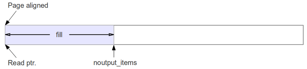
We have one thing going for us, though: all buffers are page-aligned at the start. This is great since a page alignment is good enough for any current or foreseeable SIMD alignment requirement (16 or 32 bytes right now, and when we get to the problem of requiring more than 4k alignments, I'll be happy enough to readdress the problem then). So the first call to work on a buffer is always aligned. 


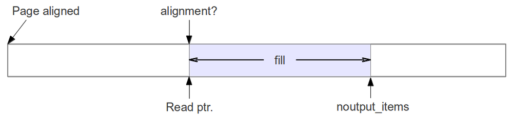
But what if the work function is called with a number of items that breaks the alignment? What are we supposed to do then?


The first attempt at a solution was to use the concept of setting a set_output_multiple value for the block. This call tells the scheduler that the block can only handle chunks of data that contain a number of items that is a multiple of this value. So if we have floats in SSE chips, we need a multiple of 4 floats per call to the work function. It will never be called with less than 4 or some odd number that will ruin our alignment. 


But there's a problem with that approach. The scheduler doesn't really function well when given that restriction. Specifically, there are two issues. First, if the data stream being processed is finite and that number is not a multiple of what's required by the alignment, then the last number of items won't ever be processed. That's not the biggest deal in the world as GNU Radio is typically meant to stream data, but it could be a problem for many applications of processing data from a file.


The second problem, though, is latency. When processing packetized data, we cannot produce a packet until we have enough samples to make the packet. But at some point, we have the last few samples sitting in the buffer waiting to be processed. Because of our output multiple restriction, we leave those sitting behind until more samples are available so that the scheduler can pass them on. That would mean a fairly large amount of added latency to handle a packet, and that's unacceptable.


No, what we need is a solution that keeps the data flowing as best as it can while still working towards keeping the buffers aligned.


Branch Location

This post discusses issues that will hopefully be merged into the main source code of GNU Radio soon. However, I would like it to undergo significant testing, first, and so have only published a branch at:

http:github.com/trondeau/gnuradio.git

as the branch safe_align.

Scheduler Alignment

Instead of using the set_output_multiple approach, we need a solution that meets the following goals:

  • Minimize effect to latency; maximize throughput.
  • Try to maintain alignment of buffers whenever possible.
  • When not possible to keep alignment, pass on data quickly.
    • minimize latency accrued by holding data.
  • Re-establish alignment but not at the expense of extra calls.
    • pass on the largest buffer possible that re-establishes alignment.
    • don't pass the minimum required. The extra overhead of calling a purposefully-truncated work function is greater than the benefit of realigning quickly.

In it's implementation, we want to minimize any added computation to the scheduler and slow down our code.


In the approach that we came up with, the scheduler looks at the number of items it has available for the block. If there are enough items to keep the buffers aligned, it passes on the largest number of samples possible that maintains the alignment. If there aren't enough, then it sends them along anyway, but it sets a flag that tells the block of the alignment problem.


When the buffers are misaligned, the scheduler must try to correct the alignment. There are two ways of doing this. The easiest way is just to pass on the minimum number of items possible that re-establishes alignment. The problem with this approach is that the number is really small, so you are asking the work function to handle 1, 2, or 3 items, say. Then it has to go back to the scheduler and ask for more. This kind of behavior incurs a tremendous amount of overhead in that it deals more with moving the data than processing it.


The second way of handling the unalignment is to take the amount of data currently available and pass on the largest possible chunk of items that will re-establish the alignment. This forces us to handle another call to work with unaligned data, but the penalty for doing that is much less than the overhead of purposefully handling small buffers. In my experiments and analysis, most of the data comes across aligned, anyway, so these calls are minimal.


To accomplish these new rules, the GNU Radio gr_block class (which is a parent class to all blocks) has these new functions:

  void set_alignment (int multiple);

  int  alignment () const { return d_output_multiple; }

  void set_unaligned (int na);

  int unaligned () const { return d_unaligned; }

  void set_is_unaligned (bool u);

  bool is_unaligned () const { return d_is_unaligned; }


A block's work function can check it's alignment and make the proper decision on what to do based on that information. The block can test the is_unaligned() and call. If it indicates that the buffers are aligned, than the aligned Volk kernel can be called. Otherwise, it can either process the data directly or call an unaligned kernel.


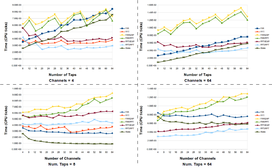
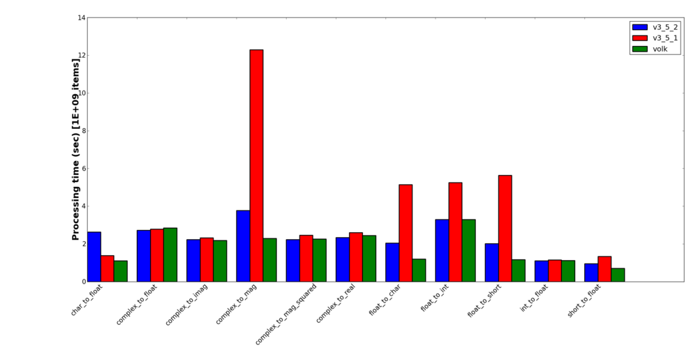
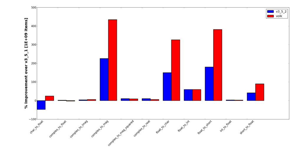
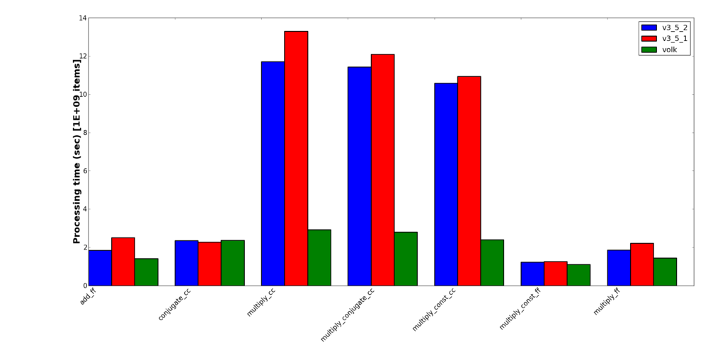
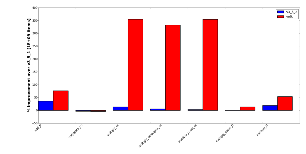
In order not to make this blog post longer than it already is, I will post a separate blog post discussing the method and results of benchmarking all of this work. In it, just to tease, I'll be showing a few surprising results. First, I'll show that the use of Volk can give us dramatic improvements for a lot of simple blocks (ok, that's not surprising). Second, on the tested processors, I see almost no penalty for making unaligned loads and stores. And third, lest you think that last claim makes all of this work unnecessary, my test show that the efforts to keep the alignment going in the new scheduler actually improves the processing speed even without using Volk. So there is a two-fold benefit to this work: one from the scheduler itself and then a second effect of Volk. 

Making Unaligned Kernels

Because we will be processing unaligned buffers in this approach, we need to either handle these cases with generic implementations or use an unaligned kernel. The generic version of the code would be like what is already in a block now that we would like to transition to using Volk. This would be the standard C/C++ for-loop math.


A useful approach, though, is to make use of unaligned Volk kernel. Even though an unaligned load is a bit more costly than an aligned call, we try to maximize the size of the buffers to process and the overall affect is still faster than a generic for loop. So it behooves us to call the unaligned version in these cases, which might mean making a new kernel specifically for this. 


Luckily, in most cases, the only difference between an aligned Volk kernel and an unaligned one is the use of loadu instead of load and storeu instead of store. These two simple differences makes it really easy to create an unaligned kernel.


With this approach, a GNU Radio block can look really simple. Let's use the gr_multiply_cc block as an example. Here's the old version of the call:

int
gr_multiply_cc::work (int noutput_items,
  gr_vector_const_void_star &input_items,
  gr_vector_void_star &output_items)
{
  gr_complex *optr = (gr_complex *) output_items[0];
  int ninputs = input_items.size ();
  for (size_t i = 0; i < noutput_items*d_vlen; i++){
    gr_complex acc = ((gr_complex *) input_items[0])[i];
    for (int j = 1; j < ninputs; j++)
      acc *= ((gr_complex *) input_items[j])[i];
    *optr++ = (gr_complex) acc;
  }
  return noutput_items;
}


That version uses a for-loop over both he number of inputs and number of items. Here's what it looks like when we call Volk.

int
gr_multiply_cc::work (int noutput_items,
     gr_vector_const_void_star &input_items,
     gr_vector_void_star &output_items)
{
  gr_complex *out = (gr_complex *) output_items[0];
  int noi = d_vlen*noutput_items;
  memcpy(out, input_items[0], noi*sizeof(gr_complex));
  if(is_unaligned()) {
    for(size_t i = 1; i < input_items.size(); i++)
      volk_32fc_x2_multiply_32fc_u(out, out, (gr_complex*)input_items[i], noi);
  }
  else {
    for(size_t i = 1; i < input_items.size(); i++)
      volk_32fc_x2_multiply_32fc_a(out, out, (gr_complex*)input_items[i], noi);
  }

  return noutput_items;
}


Here, we only loop over each input, but the calls themselves are to the Volk multiply complex kernel. We test the unaligned flag first. If the buffers are flagged as unaligned, we use the volk_32fc_x2_multiply_32fc_u kernel where the final "u" indicates that this is an unaligned kernel. So for each input stream, we process the data this way. In particular, this kernel only takes in two streams at once to multiply together, so we take the output and multiply it by the next input stream after having first pre-loaded the output buffer with the first input stream.


Now, if the block's buffers are aligned, the flag will indicate as much and the aligned version of the kernel is called. Notice that the only difference between the kernels is the "a" at the end instead of the "u" to indicate that this is an aligned kernel.


If we didn't have an unaligned kernel available, we could either create one or just call the old version of the gr_multiply_cc's work function in this case.

Blocks Converted so Far

These next few sections are starting to get really low-level and specific, so feel free to stop reading unless you are really interested in the development work. I include this as much for the historical reference as anything.


Most of these blocks that I have so far moved over to using Volk fall into the category of the "low-hanging fruit." That means that, mostly, the Volk kernels existed or were easy to create from existing Volk kernels (such as making unaligned versions of them), that the block only needed a single Volk kernel to perform the activity required, and that had very straight-forward input to output relationships.


On occasion, I went and added a few things that I thought were useful. The char->short and short->char type conversions did not exist, but they were already a Volk kernel, so making them a GNU Radio block was easy and, hopefully, useful.


I also added a gr_multiply_conjugate_cc block. This one made a lot of sense to me. First, it was really easy to add the two lines it took to convert the Volk kernel that did a complex multiply into the conjugate and multiply kernel that's there now. Since this is such an often-used function in DSP, it just seemed to make sense to have a block that did it. My benchmarking shows a notable improvement in speed by combining this operation into a single block, too. Just to note, this block takes in two (and only two) inputs where the second stream is the one that gets conjugated.


What follows is a list of blocks o different types convered to using Volk


Type conversion blocks

  • gnuradio-core/src/lib/general/gr_char_to_float
  • gnuradio-core/src/lib/general/gr_char_to_short
  • gnuradio-core/src/lib/general/gr_complex_to_xxx
  • gnuradio-core/src/lib/general/gr_float_to_char
  • gnuradio-core/src/lib/general/gr_float_to_int
  • gnuradio-core/src/lib/general/gr_float_to_short
  • gnuradio-core/src/lib/general/gr_int_to_float
  • gnuradio-core/src/lib/general/gr_short_to_char
  • gnuradio-core/src/lib/general/gr_short_to_float


Filtering blocks

  • gnuradio-core/src/lib/filter/gr_fft_filter_ccc
  • gnuradio-core/src/lib/filter/gr_fft_filter_fff
  • gnuradio-core/src/lib/filter/gri_fft_filter_ccc_generic
  • gnuradio-core/src/lib/filter/gri_fft_filter_fff_generic


General math blocks

  • gnuradio-core/src/lib/general/gr_add_ff
  • gnuradio-core/src/lib/general/gr_conjugate_cc
  • gnuradio-core/src/lib/general/gr_multiply_cc
  • gnuradio-core/src/lib/general/gr_multiply_conjugate_cc
  • gnuradio-core/src/lib/general/gr_multiply_const_cc
  • gnuradio-core/src/lib/general/gr_multiply_conjugate_cc
  • gnuradio-core/src/lib/general/gr_multiply_const_cc
  • gnuradio-core/src/lib/general/gr_multiply_const_ff
  • gnuradio-core/src/lib/general/gr_multiply_ff

Gengen to General

One thing that might confuse people who have previously developed in the guts of GNU Radio is how I moved some of the blocks from gengen to general. Many GNU Radio blocks perform some function, like basic mathematical operations on two or more streams, that behave identically from a code standpoint but which use different data types. These have been put into the gengen directory as templated files where a Python script is used to autogenerate the type-specific class. This was before Swig would properly handle actual C++ templates, so we were left doing it this way.


Well, with Volk, we don't really have the option to template classessince the Volk call is highly specific to the data type used. So when moving certain math block for a specific type out of gengen, we went with the simple solution of removing that data type from the autogeneration scripts and placing it into general as a stand-alone block that can call the right Volk function. Good examples are the gr_multiply_cc and gr_multiply_ff blocks to see what I mean.


This really seems like the simplest possible answer to the problem. It maintains our block structure that we've been using for almost a decade now and keeps things clean and simple for both developers and users. The downside is some duplication of code, but with the Volk C functions, that is somewhat inevitable and not a huge issue to deal with.

"GNU Radio is Crap" and Other Such Insights

There seem to be two kinds of people that I meet when talking about GNU Radio. Those who loves it and those who hate it. I rarely get anyone either in between or who just want to know more about it. I am writing this to explore why this happens and why some people think GNU Radio is, as is often put, crap. 

First, let me take a step back. I was recently at the Software Radio Implementation Forum (SRIF) in Hong Kong to give a talk on GNU Radio. There were some enthusiastic people in the audience who I talked to afterwards about the project. Also there was a talk on Microsoft's Sora project, another software radio system. The presentation was very enlightening, especially in regards to identifying the differences between GNU Radio and Sora. In large part, we have come at things from two completely different philosophies, which I think plays into the main thread of this article.

GNU Radio has always been about enabling the development and experimentation of communications. It was designed around the flow graph and the block structure to piece radios together. We wanted developers and designers. As such, we spent little time working on grand applications and demonstrations of the project, save maybe for the original ATSC decoder. We have lots of examples, but most of them are about how to use GNU Radio, not about showing what GNU Radio can do. There's a subtle but important difference between the two.

Sora, on the other hand, came at things with the intent of building and showing off complex applications in software radio, ostensibly to prove that GPPs could handle complex waveforms. Their initial project enabled them to do 802.11 in real-time. They then moved to LTE. Their use of memory and look-up tables to replace computations and their initial focus on using SIMD programming for speed have made a very fast, solidly performing SDR system. But it is really only now that they are building Sora into a project for developers. At this SRIF talk, I heard about them building "bricks," which we would call "blocks," that will fit together and create a radio. 

Now, this is, obviously, my take on the history of the project from the presentations and papers that I have seen and read. 

So the way that I see it is that the projects came from different directions. We started with the development and programming model, but lack good applications to showcase our product. They have great apps, but are just now getting things together as a developers platform. This represents two different mindsets that I see in the computer and programming community as a whole. There are those who want to develop and those who want to use. In a very basic and non-nuanced sense, these attitudes are the distinction between Windows users and Linux users. Linux users don't mind getting their hands dirty and working a bit harder for the freedoms and power Linux gives them. Windows users are more interested in using computers. (I confess that such as simplified comparison makes me feel like a bad stand-up comic, but I hope the point is made without belaboring the subject).

From this perspective, those people who think GNU Radio is crap, when I get a chance to talk to them about their problems, tend to be from the application side of things. They try to use one of our examples out of the box and treat it as though it is meant to be a full-on application. Except that they are examples of how to do things. We have not yet built a real digital communications application as part of GNU Radio. Our benchmark scripts are meant for benchmarking and exploring how to do digital communications. They were never meant to be used as part of a deployed communications platform. If you look at it, we don't even use equalizers or channel coding, so they are fragile and hard to use. But we've never claimed any differently.

Still, our examples are there for the world to see, and I can't be surprised when people mistake the intentions. And so I similarly cannot be upset when I get the reactions from people who wanted to use GNU Radio to make an quick application based on OFDM or MIMO. We simply haven't provided them with the means to do so.

On the other hand, when someone comes to the project with a developers mindset and wants to do something complicated, they can spend the time to work with the code and see what kind of capabilities are offered. We have some great developers who have done some amazing things with GNU Radio, and so we know that it's not crap. But it's not shiny, either.

To conclude, I'm left with the difficult problem of trying to think if there is a way to solve this problem. There is definitely no single solution or magic bullet. I'd love to see evne more complete applications get published on CGRAN or sites like Github. And for some of those that are already published, some amount of care needs to be taken to ensure some quality control, by which I mean good documentation and a user interface to the products as well as easy maintanence as GNU Radio versions evolve. I'd also love more feedback and additions to our examples in GNU Radio, even to the extent that we can get more of what we would call applications (there's a reason we have an examples and apps directory in our new tree

structure). These ideas involve the buy-in of the community and a slight change in our ideas and understanding of how to construct and present applications to the world.

SNR Estimators

In GNU Radio, we have been slowly evolving our digital communications capabilities. One thing that becomes quickly and painfully obvious to anyone doing real over-the-air communications with digital modulations is that the modulators and demodulators are the easy part. It's the synchronization that's the hard part and where most of your work as a designer goes.

Generally speaking, synchronization means three (maybe four) things: frequency, timing, and phase. The fourth is automatic gain control (AGC). While AGC isn't really "synchronization," it follows similar principles of an adaptive loop. Different modulation schemes have different methods for AGC and synchronization. These tend to fall into categories of narrowband, wideband (and then ultrawideband), and OFDM, but we can easily dispense with these categories and go in depth into differences within them, too. For instance, narrowband PSK and FSK systems have pretty widely different requirements out of a receiver for demodulation and the appropriate synchronization algorithms reflect this.

But this post is about SNR estimation. The reason to talk about synchronization here it twofold. First, like synchronizers, SNR estimation techniques can vary widely depending on the modulation scheme being used. Second, most synchronization schemes like to be reactive to changes in SNR. You can often find different algorithms that work well in low SNR cases but not high, or they are too costly to perform in high SNR where the signal quality allows you to use something simpler and/or more accurate. Take for example an equalizer. The constant modulus equalizer is great for PSK signals, but we know that an LMS decision-directed equalizer works better. But a decision-directed equalizer only works in cases where the SNR is large enough that the majority of samples are correct. So we often start with a blind CMA for acquisition purposes and then move to a decision-directed approach once we've properly locked on to the signal.

We've been meaning to add SNR estimators to GNU Radio for some time, now, and I finally developed enough of an itch to start doing it. But as I said, each modulation could use a different equalizer, and there are various equalizers designed for this modulation in that channel or that modulation in such and such channel. If you have access to IEEExplore, a simple search for "snr estimator" produces 1,279 results. Now, I know that's nothing to a Google search, but twelve hundred scholarly (we hope) articles on a topic is a lot to get through, and you will quickly see that there are finely-tuned estimators for different modulations and channels.

What I did was give us a start into this area. I took a handful of the most generic, computationally realistic estimators that I could find for PSK signals and implemented them. I'll give a shout out here to Normon Beaulieu, who has written a lot in this field. I've found that a lot of his work in SNR estimators to be accessible and useful, and he presents his work in ways that can be easily translated into actual, working code.

I also took the tack of looking for estimators that worked in AWGN channels. Now, if you've ever heard me speak on the subject of communications education or research, you've probably heard me scoff at anyone who develops a system under simulated AWGN conditions. In the case of an SNR estimator, though, I thought about this and had to come to the conclusion that the only way to handle this is to have an estimator that you can plug in variables for your channel model, which of course assumes that you have or can estimate these parameters. So in the end, I followed Beaulieu's lead in at least one of this papers and took algorithms that could be both simplified and tested by assuming AWGN conditions. I did, however, provide one of these algorithms (what I refer to as the M2M4 algorithm) in a way that allows a user to specify parameters to better fit a non-AWGN channel and non-PSK signals. Using the AWGN-based algorithms with this other version of the M2M4 seemed like a good compromise for being computable without more information but at least providing a tip of my hat to the issue of non-AWGN channels. If nothing else, these estimators should give us a ballpark estimate.

I also specifically developed these estimators based on a parent class that would easily allow us to add more estimators as they are developed. Right now, the parent class is specifically for MPSK, but we can add other estimator parent classes for other modulations; maybe have them all inherit from a single class in the end -- this is fine, since the inheritance would really be hidden from the end user. The class itself is in the gr-digital component and called digital_impl_mpsk_snr_est. It's constructor is simply:

digital_impl_mpsk_snr_est(double alpha);

Where the parameter alpha is the value used in a running average as every estimator I've seen is based on expected values of a time series, which we estimate with the running average. This value defaults to 0.001 and should be kept small.

I have created four estimators that inherit from this block. These are named the "simple," "skew," "M2M4," and "SVR" estimators. The last two come from [1]. The "skew" estimator uses a skewness measure that was developed in conversation with fred harris. The simple estimator is probably written up and documented somewhere, but it's the typical measurement based on the mean and variance of the constellation cloud.  I've tried to document these as best as possible in the header files themselves, so I'll refer you to the Doxygen documentation for details (note that as of the writing of this blog post, these estimators are only in the Git repository but will be available starting in the 3.5.1 release). The "SNR estimators"  group in the Doxygen manual can be used to find all of the available estimators and details about how to use them.

In particular, the M2M4 and SVR methods were developed around fading channels and both use the kurtosis of the modulation signal (k_a) and kurtosis of the channel (k_w) in their calculations. This is great if these values are know or can be estimated. In the case of the M2M4 algorithm, I provide a version of it, called the digital_impl_snr_est_m2m4, as an example of a non-PSK and non-AWGN method; right now, this block is unavailable through any actual GNU Radio block. It's untested and unverified, but I wanted it there for reference and hopefully to use later.


SNR Use in Demodulation

The main intent of having an SNR estimator block is to enable the use of SNR information by other blocks. As such, there are two GNU Radio blocks that are defined for doing this in different ways. First off, let's say that the SNR estimation is done after timing recovery (see harris' paper "Let’s Assume the System is Synchronized", which is unfortunately fairly costly but worth it if you can get a copy). So in GNU Radio terms, this means that the SNR is estimated down stream of most of the synchronization blocks. While I would like to just pass a tag along with the SNR information, that does won't work for every block, like the frequency recovery, AGC, and timing recovery loops that come before. Instead, we will have to pass them a message with this information. However, some blocks exist downstream that want this info, too, like the channel equalizer.

To accommodate both possible uses, I created two blocks. The digital_mpsk_snr_est_cc block is a flowgraph with a single input and single output port, so it's meant to go inline in a flowgraph. This block produces tags with the SNR every N samples, where N is set by the user (the second arg in the constructor and through the set_tag_nsamples(int N) function). The downstream blocks can then look for the tag with the key "snr" and pull out this information when they need it. The value of N defaults to 10,000 as an arbitrary, fairly large number. You'll want to set this depending on the speed you expect the SNR conditions to change.

The second block is a probe, which is GR speak for a sink. It's called digital_probe_mpsk_snr_est_c and only takes a single complex input stream. Right now, it just acts as a sink where the application running the flow graph can query the SNR by calling the "snr()" function on this block (the same is true for the digital_mpsk_snr_est_cc block, too). However, this block uses a similar constructor in that you set a value N for the number of samples between messages. In this case, instead of sending a tag down stream, it will send a message every N samples. The problem with this is that our message passing system isn't really advanced or easy enough to use to set this up properly. Recent work by Josh Blum might fix this, though.

Eventually, though, we hope to be able to create flow graphs where the SNR estimation is passed around to other blocks to allow them to adjust their behavior. In the case I'm interested in right now, I'd like to pass this info to the frequency lock loop to stop it if the SNR falls below a certain level so that it doesn't walk away when there is no signal to acquire.


[1]  D. R. Pauluzzi and N. C. Beaulieu, "A comparison of SNR estimation techniques for the AWGN channel," IEEE Trans. Communications, Vol. 48, No. 10, pp. 1681-1691, 2000.